I recently wrapped up a version of my
R function for easy Bayesian bootstrappin’ into the package bayesboot. This package implements a function, also named bayesboot, which performs the Bayesian bootstrap introduced by Rubin in 1981. The Bayesian bootstrap can be seen as a smoother version of the classical non-parametric bootstrap, but I prefer seeing the classical bootstrap as an approximation to the Bayesian bootstrap :)
The implementation in bayesboot can handle both summary statistics that works on a weighted version of the data (such as weighted.mean) and that works on a resampled data set (like median). As bayesboot just got accepted on CRAN you can install it in the usual way:
For the third year round I and
Ullrika Sahlin arranged
Bayes@Lund, a mini-conference bringing together researchers interested in or working with Bayesian methods in and around Sweden. This year we were thrilled to have over 70 attendees, both from near and far, perhaps due to our interesting invited speakers
Eric-Jan Wagenmakers and
Robert Grant, or perhaps due to the promise of fika (a Swedish word referring to a break involving coffee and/or tea with cake and/or cookies and/or pastries, the more and the better). Perhaps it was a combination…
Bayesian data analysis is cool, Markov chain Monte Carlo is the cool technique that makes Bayesian data analysis possible, and wouldn’t it be coolness if you could do all of this in the browser? That was what I thought, at least, and I’ve now made
bayes.js: A small JavaScript library that implements an adaptive MCMC sampler and a couple of probability distributions, and that makes it relatively easy to implement simple Bayesian models in JavaScript.
Here is a motivating example: Say that you have the heights of the last ten American presidents…
// The heights of the last ten American presidents in cm, from Kennedy to Obama
var heights = [183, 192, 182, 183, 177, 185, 188, 188, 182, 185];
… and that you would like to fit a Bayesian model assuming a Normal distribution to this data. Well, you can do that right now by clicking “Start sampling” below! This will run an MCMC sampler in your browser implemented in JavaScript.
If this doesn’t seem to work in your browser, for some reason, then try
this version of the demo.
Christmas is soon upon us and here are some gift ideas for your statistically inclined friends (or perhaps for you to put on your own wish list). If you have other suggestions please leave a comment! :)
1. Games of probability
A recently released game where probability takes the main role is
Pairs, an easy going press-your-luck game that can be played in 10 minutes. It uses a custom “triangular” deck of cards (1x1, 2x2, 3x3, …, 10x10) and is a lot of fun to play, highly recommended!
On the 21st of February, 2015, my wife had not had her period for 33 days, and as we were trying to conceive, this was good news! An average period is around a month, and if you are a couple trying to go triple, then a missing period is a good sign something is going on. But at 33 days, this was not yet a missing period, just a late one, so how good news was it? Pretty good, really good, or just meh?
To get at this I developed a simple Bayesian model that, given the number of days since your last period and your history of period onsets, calculates the probability that you are going to be pregnant this period cycle. In this post I will describe what data I used, the priors I used, the model assumptions, and how to fit it in R using importance sampling. And finally I show you why the result of the model really didn’t matter in the end. Also I’ll give you a handy script if you want to calculate this for yourself. :)
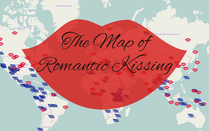
Romantic kissing is a cultural universal, right? Nope! At least not if you are to believe Jankowiak et al. (2015) who surveyed a large number of cultures and found that “sexual-romantic kissing” occurred in far from all of them. For some reasons the paper didn’t include a world map with these kissers and non-kissers plotted out. So, with the help of my colleague Andrey Anikin I’ve now made such a map using R and
the excellent leaflet package. Click on the image below to check it out:
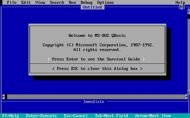
The BASIC programming language was at one point the most widely spread programming language. Many home computers in the 80s came with BASIC (like the Commodore 64 and the Apple II), and in the 90s both DOS and Windows 95 included a copy of the
QBasic IDE. QBasic was also the first programming language I encountered (I used it to write a couple of really horrible text adventures). Now I haven’t programmed in BASIC for almost 20 years and I thought I would revisit this (from my current perspective) really weird language. As I spend a lot of time doing Bayesian data analysis, I though it would be interesting to see what a Bayesian analysis would look like if I only used the tool that I had 20 years ago, that is, BASIC.
This post walks through the implementation of the Metropolis-Hastings algorithm, a standard Markov chain Monte Carlo (MCMC) method that can be used to fit Bayesian models, in BASIC. I then use that to fit a Laplace distribution to the most adorable dataset that I could find: The number of wolf pups per den from a sample of 16 wold dens. Finally I summarize and plot the result, still using BASIC. So, the target audience of this post is the intersection of people that have programmed in BASIC and are into Bayesian computation. I’m sure you are out there. Let’s go!
This is a screencast of my
UseR! 2015 presentation: Tiny Data, Approximate Bayesian Computation and the Socks of Karl Broman. Based on
the original blog post it is a quick’n’dirty introduction to approximate Bayesian computation (and is also, in a sense, an introduction to Bayesian statistics in general). Here it is, if you have 15 minutes to spare:
A while back I wrote about
how the classical non-parametric bootstrap can be seen as a special case of the Bayesian bootstrap. Well, one difference between the two methods is that, while it is straightforward to roll a classical bootstrap in R, there is no easy way to do a Bayesian bootstrap. This post, in an attempt to change that, introduces a bayes_boot function that should make it pretty easy to do the Bayesian bootstrap for any statistic in R. If you just want a function you can copy-n-paste into R go to
The bayes_boot function below. Otherwise here is a quick example of how to use the function, followed by some details on the implementation.
Update: I’ve now created an R package that implements the Bayesian bootstrap, which I recommend instead of using the function described in this post. You can install it by running install.packages("bayesboot") in R and you can read more about it
here. The implementation is the same as here, but the interface is slightly different.
hygge A Danish word (pronounced HU-guh) meaning social coziness. I.e. the feeling of a good social atmosphere. –
Urban Dictionary
Yes, there was plenty of hygge to go around this year’s UseR! that took place last week in Aalborg, Denmark. Everybody I’ve spoken with agrees that it was an extraordinary conference, from the interesting speakers and presentations to the flawless organization (spearheaded by
Torben Tvedebrink) and the warm weather. As there were many parallel session, I only managed to attend a fraction of the talks, but here are some of my highlights: