Hello stranger, and welcome! 👋😊
I'm Rasmus Bååth, data scientist, engineering manager, father, husband, tinkerer,
tweaker, coffee brewer, tea steeper, and, occasionally, publisher of stuff I find
interesting down below👇
In
a previous post I used the
the Million Base 2.2 chess data base to calculate the predictive piece values of chess pieces. It worked out pretty well and here, just for fun, I thought I would check out what happens with the predictive piece values over the course of a chess game. In the previous analysis, the data (1,000,000 chess positions) was from all parts of the chess games. Here, instead, are the predictive piece values using only positions up to the 10th first full moves (a full move is when White and Black each have made a move):
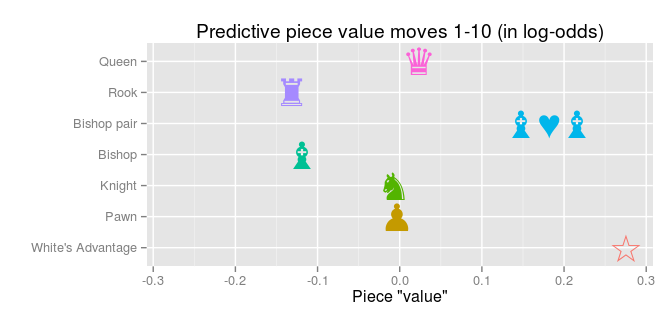
Who doesn’t like chess? Me! Sure, I like the idea of chess – intellectual masterminds battling each other using nothing but pure thought – the problem is that I tend to lose, probably because I don’t really know how to play well, and because I never practice. I do know one thing: How much the different pieces are worth, their point values:

This was among the first things I learned when I was taught chess by my father. Given these point values it should be as valuable to have a knight on the board as having three pawns, for example. So where do these values come from? The point values are not actually part of the rules for chess, but are rather just used as a guideline when trading pieces, and they seem to be based on the expert judgment of chess authorities. (According to the guardian of truth
there are many alternative valuations, all in the same ballpark as above.) As I recently learned that it is very important to be able to write Big Data on your CV, I decided to see if these point values could be retrieved using zero expert judgement in favor of huge amounts of chess game data.
The non-parametric bootstrap was my first love. I was lost in a muddy swamp of zs, ts and ps when I first saw her. Conceptually beautiful, simple to implement, easy to understand (I thought back then, at least). And when she whispered in my ear, “I make no assumptions regarding the underlying distribution”, I was in love. This love lasted roughly a year, but the more I learned about statistical modeling, especially the Bayesian kind, the more suspect I found the bootstrap. It is most often explained as a procedure, not a model, but what are you actually assuming when you “sample with replacement”? And what is the underlying model?
Still, the bootstrap produces something that looks very much like draws from a posterior and there are papers comparing the bootstrap to Bayesian models (for example,
Alfaro et al., 2003).
Some also wonder which alternative is more appropriate: Bayes or bootstrap? But these are not opposing alternatives, because the non-parametric bootstrap is a Bayesian model.
In this post I will show how the classical non-parametric bootstrap of
Efron (1979) can be viewed as a Bayesian model. I will start by introducing the so-called Bayesian bootstrap and then I will show three ways the classical bootstrap can be considered a special case of the Bayesian bootstrap. So basically this post is just a rehash of
Rubin’s The Bayesian Bootstrap from 1981. Some points before we start:
-
Just because the bootstrap is a Bayesian model doesn’t mean it’s not also a frequentist model. It’s just different points of view.
-
Just because it’s Bayesian doesn’t necessarily mean it’s any good. “We used a Bayesian model” is as much a quality assurance as “we used probability to calculate something”. However, writing out a statistical method as a Bayesian model can help you understand when that method could work well and how it can be made better (it sure helps me!).
-
Just because the bootstrap is sometimes presented as making almost no assumptions, doesn’t mean it does. Both the classical non-parametric bootstrap and the Bayesian bootstrap make very strong assumptions which can be pretty sensible and/or weird depending on the situation.
Everybody loves speed comparisons! Is R faster than Python? Is dplyr faster than data.table? Is STAN faster than JAGS? It has been said that speed comparisons are utterly meaningless, and in general I agree, especially when you are comparing apples and oranges which is what I’m going to do here. I’m going to compare a couple of alternatives to lm(), that can be used to run linear regressions in R, but that are more general than lm(). One reason for doing this was to see how much performance you’d loose if you would use one of these tools to run a linear regression (even if you could have used lm()). But as speed comparisons are utterly meaningless, my main reason for blogging about this is just to highlight a couple of tools you can use when you grown out of lm(). The speed comparison was just to lure you in. Let’s run!

For the second year round I and
Ullrika Sahlin arranged the mini-conference Bayes@Lund, with the aim of bringing together researchers in the south of Sweden working with Bayesian methods. This year the committee was also beefed up by
Paul Caplat and
Krzysztof Podgorski. What originally made me and Ullrika start this get-together is our feeling that Lund University is lagging behind with regards to Bayesian methods (we don’t have a single introductory course on Bayes stats!) and that we need a venue where people doing Bayes can meet and discuss what cool stuff they are working on. And so, last Tuesday, over 60 researchers got together to listen to twelve interesting talks, discuss, and (not least) fika. Here follows some highlights from Bayes@Lund 2015.

“Behind every great point estimate stands a minimized loss function.” – Me, just now
This is a continuation of Probable Points and Credible Intervals, a series of posts on Bayesian point and interval estimates. In
Part 1 we looked at these estimates as graphical summaries, useful when it’s difficult to plot the whole posterior in good way. Here I’ll instead look at points and intervals from a decision theoretical perspective, in my opinion the conceptually cleanest way of characterizing what these constructs are.
If you don’t know that much about Bayesian decision theory, just chillax. When doing Bayesian data analysis you get it
“pretty much for free” as esteemed statistician Andrew Gelman puts it. He then adds that it’s “not quite right because it can take effort to define a reasonable utility function.” Well, perhaps not free, but it is still relatively straight forward! I will use a toy problem to illustrate how Bayesian decision theory can be used to produce point estimates and intervals. The problem is this: Our favorite droid has gone missing and we desperately want to find him!

Peter Norvig, the director of research at Google, wrote a nice essay on
How to Write a Spelling Corrector a couple of years ago. That essay explains and implements a simple but effective spelling correction function in just 21 lines of Python. Highly recommended reading! I was wondering how many lines it would take to write something similar in base R. Turns out you can do it in (at least) two pretty obfuscated lines:
sorted_words <- names(sort(table(strsplit(tolower(paste(readLines("https://www.norvig.com/big.txt"), collapse = " ")), "[^a-z]+")), decreasing = TRUE))
correct <- function(word) { c(sorted_words[ adist(word, sorted_words) <= min(adist(word, sorted_words), 2)], word)[1] }
While not working exactly as Norvig’s version it should result in similar spelling corrections:
## [1] "piece"
## [1] "of"
## [1] "cake"

So let’s deobfuscate the two-liner slightly (however, the code below might not make sense if you don’t read
Norvig’s essay first):
Making a slight digression from last month’s
Probable Points and Credible Intervals here is how to summarize a 2D posterior density using a highest density ellipse. This is a straight forward extension of the highest density interval to the situation where you have a two-dimensional posterior (say, represented as a two column matrix of samples) and you want to visualize what region, containing a given proportion of the probability, that has the most probable parameter combinations. So let’s first have a look at a fictional 2D posterior by using a simple scatter plot:

Whoa… that’s some serious over-plotting and it’s hard to see what’s going on. Sure, the bulk of the posterior is somewhere in that black hole, but where exactly and how much of it?
Why R? Because S!
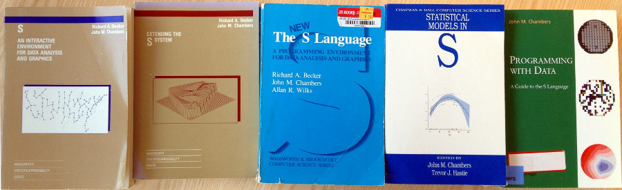
R is the open source implementation (and a pun!) of S, a language for statistical computing that was developed at Bell Labs in the late 1970s. After that, the implementation of S underwent a number of major revisions documented in a series of seminal books, often just referred to by the color of their cover: The Brown Book, the Blue Book, the White Book and the Green Book. To satisfy my techno-historical lusts I recently acquired all these books and I though I would share some tidbits from them, highlighting how S (and thus R) developed into what we today love and cherish. But first, here are the books in chronological order from left to right:
After having broken the Bayesian eggs and prepared your model in your statistical kitchen the main dish is the posterior. The posterior is the posterior is the posterior, given the model and the data it contains all the information you need and anything else will be a little bit less nourishing. However, taking in the posterior in one gulp can be a bit difficult, in all but the most simple cases it will be multidimensional and difficult to plot. But even if it is one-dimensional and you could plot it (as, say, a density plot) that does not necessary mean that it is easy to see what’s going on.
One way of getting around this is to take a bite at a time and look at summaries of the marginal posteriors of the variables of interest, the two most common type of summaries being point estimates and credible intervals (an interval that covers a certain percentage of the probability distribution). Here one is faced with a choice, which of the many ways of constructing point estimates and credible intervals to choose? This is a perfectly good question that can be given an unhelpful answer (with a predictable follow-up question):
- That depends on your loss function.
- So which loss function should I use?