A while back I wrote about
how the classical non-parametric bootstrap can be seen as a special case of the Bayesian bootstrap. Well, one difference between the two methods is that, while it is straightforward to roll a classical bootstrap in R, there is no easy way to do a Bayesian bootstrap. This post, in an attempt to change that, introduces a bayes_boot function that should make it pretty easy to do the Bayesian bootstrap for any statistic in R. If you just want a function you can copy-n-paste into R go to
The bayes_boot function below. Otherwise here is a quick example of how to use the function, followed by some details on the implementation.
Update: I’ve now created an R package that implements the Bayesian bootstrap, which I recommend instead of using the function described in this post. You can install it by running install.packages("bayesboot") in R and you can read more about it
here. The implementation is the same as here, but the interface is slightly different.
A quick example
So say you scraped
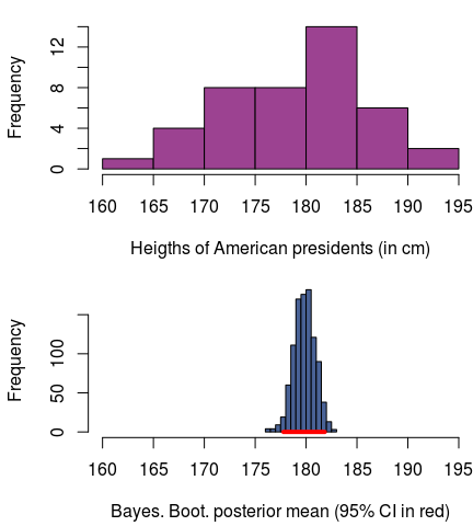
the heights of all the U.S. Presidents off Wikipedia (american_presidents.csv) and you want to run a Bayesian bootstrap analysis on the mean height of U.S. Presidents (don’t ask me why you would want to do this). Then, using the bayes_boot function
found below, you can run the following:
presidents <- read.csv("american_presidents.csv")
bb_mean <- bayes_boot(presidents$height_cm, mean, n1 = 1000)
Here is how to get a 95% credible interval:
quantile(bb_mean, c(0.025, 0.975))
##  2.5% 97.5%
## 177.8 181.8
And, of course, we can also plot this:
(Here, and below, I will save you from the slightly messy plotting code, but if you really want to see it you can check out the full script here.)
Now, say we want run a linear regression on presidential heights over time, and we want to use the Bayesian bootstrap to gauge the uncertainty in the regression coefficients. Then we will have to do a little more work, as the second argument to bayes_boot should be a function that takes the data as the first argument and that returns a vector of parameters/coefficients:
bb_linreg <- bayes_boot(presidents, function(data) {
  lm(height_cm ~ order, data)$coef
}, n1 = 1000)
Ok, so it is not really over time, as we use the order of the president as the predictor variable, but close enough. Again, we can get a 95% credible interval of the slope:
quantile(bb_linreg$order, c(0.025, 0.975))
##    2.5%   97.5%
## 0.03979 0.34973
And here is a plot showing the mean posterior regression line with a smatter of lines drawn from the posterior to visualize the uncertainty:
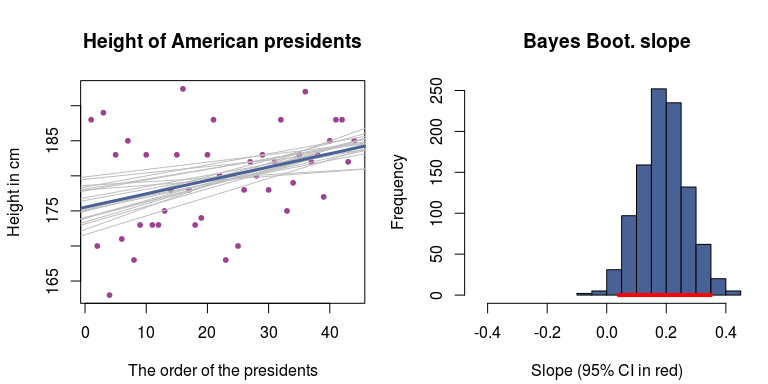
Given the model and the data, the average height of American presidents increases by around 0.2 cm for each president elected to office. So, either we have that around the 130th president the average height of presidents will be around 2 meters (≈ 6'7’’), or perhaps a linear regression isn’t really a reasonable model here… Anyhow, it was easy to do the Bayesian bootstrap! :)
How to implement a Bayesian bootstrap in R
It is possible to characterize the statistical model underlying the Bayesian bootstrap in a couple of different ways, but all can be implemented by the same computational procedure:
To generate a Bayesian bootstrap sample of size n1, repeat the following n1 times:
- Draw weights from a uniform Dirichlet distribution with the same dimension as the number of data points.
- Calculate the statistic, using the Dirichlet draw to weight the data, and record it.
1. Drawing weights from a uniform Dirichlet distribution
One way to characterize drawing from an n-dimensional uniform Dirichlet distribution is as drawing a vector of length n where the values are positive, sum to 1.0, and where any combination of values is equally likely. Another way to characterize a uniform Dirichlet distribution is as a uniform distribution over the unit simplex, where a unit simplex is a generalization of a triangle to higher dimensions, with sides that are 1.0 long (hence the unit). The figure below pictures the one, two, three and four-dimensional unit simplex:

Image source:
Introduction to Discrete Differential Geometry by
Peter Schröder
Drawing from an n-dimensional uniform Dirichlet distribution can be done by drawing $\text{Gamma(1,1)}$ distributed numbers and normalizing these to sum to 1.0 (
source). As a $\text{Gamma(1,1)}$ distribution is the same as an $\text{Exponential}(1)$ distribution, the following two lines of R code implements drawing n1 draws from an n dimensional uniform Dirichlet distribution:
dirichlet_sample <- matrix( rexp(n * n1, 1) , ncol = n, byrow = TRUE)
dirichlet_sample <- dirichlet_sample / rowSums(dirichlet_sample)
With n <- 4 and n1 <- 3 you could, for example, get:
##         [,1]    [,2]   [,3]    [,4]
## [1,] 0.61602 0.06459 0.2297 0.08973
## [2,] 0.05384 0.12774 0.4685 0.34997
## [3,] 0.17419 0.42458 0.1649 0.23638
2. Calculate the statistic using a Dirichlet draw to weight the data
Here is where, if you were doing a classical non-parametric bootstrap, you would use your resampled data to calculate a statistic (say a mean). Instead, we will want to calculate our statistic of choice using the Dirichlet draw to weight the data. This is completely straightforward if the statistic can be calculated using weighted data, which is the case for weighted.mean(x, w) and lm(..., weights). For the many statistics that do not accept weights, such as median and cor, we will have to perform a second sampling step where we (1) sample from the data according to the probabilities defined by the Dirichlet weights, and (2) use this resampled data to calculate the statistic. It is important to notice that we here want to draw an as large sample as possible from the data, and not a sample of the same size as the original data. The point is that the proportion of times a datapoint occurs in this resampled dataset should be roughly proportional to that datapoint’s weight.
Note that doing this second resampling step won’t work if the statistic changes with the sample size! An example of such a statistic would be the sample standard deviation (sd), population standard deviation would be fine, however
Bringing it all together
Below is a small example script that takes the presidents dataset and does a Bayesian Bootstrap analysis of the median height. Here n1 is the number of bootstrap draws and n2 is the size of the resampled data used to calculate the median for each Dirichlet draw.
n1 <- 3000
n2 <- 1000
n_data <- nrow(presidents)
# Generating a n1 by n_data matrix where each row is an n_data dimensional
# Dirichlet draw.
weights <- matrix( rexp(n_data * n1, 1) , ncol = n_data, byrow = TRUE)
weights <- weights / rowSums(weights)

bb_median <- rep(NA, n1)
for(i in 1:n1) {
  data_sample <- sample(presidents$height_cm, size = n2, replace = TRUE, prob = weights[i,])
  bb_median[i] <- median(data_sample)
}

# Now bb_median represents the posterior median height, and we can do all
# the usual stuff, like calculating a 95% credible interval.
quantile(bb_median, c(0.025, 0.975))
##  2.5% 97.5%
##   178   183
If we were interested in the mean instead, we could skip resampling the data and use the weights directly, like this:
bb_mean <- rep(NA, n1)
for(i in 1:n1) {
  bb_mean[i] <- weighted.mean(presidents$height_cm, w = weights[i,])
}
quantile(bb_mean, c(0.025, 0.975))
##  2.5% 97.5%
## 177.8 181.9
If possible, you will probably want to use the weight method; it will be much faster as you skip the costly resampling step. What size of the bootstrap samples (n1) and size of the resampled data (n2) to use? The boring answers are: “As many as you can afford” and “Depends on the situation”, but you’ll probably want at least 1000 of each.
The bayes_boot function
Here follows a handy function for running a Bayesian bootstrap that you can copy-n-paste directly into your R-script. It should accept any type of data that comes as a vector, matrix or data.frame and allows you to use both statistics that can deal with weighted data (like weighted.mean) and statistics that don’t (like median). See
above and
below for examples of how to use it.
Caveat: While I have tested this function for bugs, do keep an eye open and tell me if you find any. Again, note that doing the second resampling step (use_weights = FALSE) won’t work if the statistic changes with the sample size!
# Performs a Bayesian bootstrap and returns a sample of size n1 representing the
# posterior distribution of the statistic. Returns a vector if the statistic is
# one-dimensional (like for mean(...)) or a data.frame if the statistic is
# multi-dimensional (like for the coefs. of lm).
# Parameters
#   data      The data as either a vector, matrix or data.frame.
#   statistic A function that accepts data as its first argument and possibly
#             the weights as its second, if use_weights is TRUE.
#             Should return a numeric vector.
#   n1        The size of the bootstrap sample.
#   n2        The sample size used to calculate the statistic each bootstrap draw.
#   use_weights  Whether the statistic function accepts a weight argument or
#                should be calculated using resampled data.
#   weight_arg   If the statistic function includes a named argument for the
#                weights this could be specified here.
#   ...       Further arguments passed on to the statistic function.
bayes_boot <- function(data, statistic, n1 = 1000, n2 = 1000 , use_weights = FALSE, weight_arg = NULL, ...) {
  # Draw from a uniform Dirichlet dist. with alpha set to rep(1, n_dim).
  # Using the facts that you can transform gamma distributed draws into
  # Dirichlet draws and that rgamma(n, 1) <=> rexp(n, 1)
  dirichlet_weights <- matrix( rexp(NROW(data) * n1, 1) , ncol = NROW(data), byrow = TRUE)
  dirichlet_weights <- dirichlet_weights / rowSums(dirichlet_weights)

  if(use_weights) {
    stat_call <- quote(statistic(data, w, ...))
    names(stat_call)[3] <- weight_arg
    boot_sample <- apply(dirichlet_weights, 1, function(w) {
      eval(stat_call)
    })
  } else {
    if(is.null(dim(data)) || length(dim(data)) < 2) { # data is a list type of object
      boot_sample <- apply(dirichlet_weights, 1, function(w) {
        data_sample <- sample(data, size = n2, replace = TRUE, prob = w)
        statistic(data_sample, ...)
      })
    } else { # data is a table type of object
      boot_sample <- apply(dirichlet_weights, 1, function(w) {
        index_sample <- sample(nrow(data), size = n2, replace = TRUE, prob = w)
        statistic(data[index_sample, ,drop = FALSE], ...)
      })
    }
  }
  if(is.null(dim(boot_sample)) || length(dim(boot_sample)) < 2) {
    # If the bootstrap sample is just a simple vector return it.
    boot_sample
  } else {
    # Otherwise it is a matrix. Since apply returns one row per statistic
    # let's transpose it and return it as a data frame.
    as.data.frame(t(boot_sample))
  }
}
Update: Ilanfri has now ported the bayes_boot function to Python.
More examples using bayes_boot
Let’s start by drawing some fake data from an exponential distribution with mean 1.0 and compare using the following methods to infer the mean:
- The classical non-parametric bootstrap using
bootfrom thebootpackage. - Using
bayes_bootwith “two level sampling”, that is, sampling both weights and then resampling the data according to those weights. - Using
bayes_bootwith weights (use_weights = TRUE) - Assuming an exponential distribution (the “correct” distribution since we know where the data came from), with a flat prior over the mean.
First generating some data:
set.seed(1337)
exp_data <- rexp(8, rate = 1)
exp_data
## [1] 0.15 0.13 2.26 0.92 0.17 1.55 0.13 0.02
Then running the four different methods:
library(boot)
b_classic <- boot(exp_data, function(x, i) { mean(x[i])}, R = 10000)
bb_sample <- bayes_boot(exp_data, mean, n1 = 10000, n2 = 1000)
bb_weight <- bayes_boot(exp_data, weighted.mean, n1 = 10000, use.weights = TRUE, weight_arg = "w")

# Just a hack to sample from the posterior distribution when
# assuming an exponential distribution with a Uniform(0, 10) prior
prior <- seq(0.001, 10, 0.001)
post_prob <- sapply(prior, function(mean) { prod(dexp(exp_data, 1/mean)) })
post_samp <- sample(prior, size = 10000, replace = TRUE, prob = post_prob)
Here are the resulting posterior/sampling distributions:
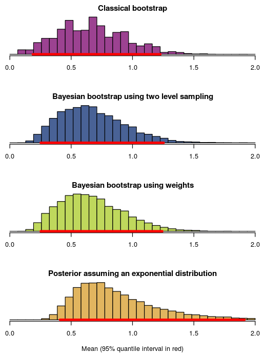
This was mostly to show off the syntax of bayes_boot, but some things to point out in the histograms above are that:
- Using the Bayesian bootstrap with two level sampling or weights result in very similar posterior distributions, which should be the case when the size of the resampled data is large (here set to
n2 = 1000). - The classical non-parametric bootstrap is pretty similar to the Bayesian bootstrap ( as we would expect).
- The bootstrap distributions are somewhat similar to the posterior mean assuming an exponential distribution, but completely misses out on the uncertainty in the right tail. This is due to the “somewhat peculiar model assumptions” of the bootstrap as critiqued by Rubin (1981)
Finally, a slightly more complicated example, where we do Bayesian bootstrap analysis of LOESS regression applied to the cars dataset on the speed of cars and the resulting distance it takes to stop. The loess function returns, among other things, a vector of fitted y values, one value for each x value in the data. These y values define the smoothed LOESS line and is what you would usually plot after having fitted a LOESS. Now we want to use the Bayesian bootstrap to gauge the uncertainty in the LOESS line. As the loess function accepts weighted data, we’ll simply create a function that takes the data with weights and returns the fitted y values. We’ll then plug that function into bayes_boot:
boot_fn <- function(cars, weights) {
  loess(dist ~ speed, cars, weights = weights)$fitted
}

bb_loess <- bayes_boot(cars, boot_fn, n1 = 1000, use_weights = TRUE, weight_arg = "weights")
To plot this takes a couple of lines more:
# Plotting the data
plot(cars$speed, cars$dist, pch = 20, col = "tomato4", xlab = "Car speed in mph",
     ylab = "Stopping distance in ft", main = "Speed and Stopping distances of Cars")

# Plotting a scatter of Bootstrapped LOESS lines to represent the uncertainty.
for(i in sample(nrow(bb_loess), 20)) {
  lines(cars$speed, bb_loess[i,], col = "gray")
}
# Finally plotting the posterior mean LOESS line
lines(cars$speed, colMeans(bb_loess, na.rm = TRUE), type ="l",
      col = "tomato", lwd = 4)

Fun fact: The cars dataset is from the 20s! Which explains why the fastest car travels at 25 mph. It would be interesting to see a comparison with stopping times for modern cars!
References
Rubin, D. B. (1981). The Bayesian Bootstrap. The annals of statistics, 9(1), 130-134. pdf