“Behind every great point estimate stands a minimized loss function.” – Me, just now
This is a continuation of Probable Points and Credible Intervals, a series of posts on Bayesian point and interval estimates. In Part 1 we looked at these estimates as graphical summaries, useful when it’s difficult to plot the whole posterior in good way. Here I’ll instead look at points and intervals from a decision theoretical perspective, in my opinion the conceptually cleanest way of characterizing what these constructs are.
If you don’t know that much about Bayesian decision theory, just chillax. When doing Bayesian data analysis you get it “pretty much for free” as esteemed statistician Andrew Gelman puts it. He then adds that it’s “not quite right because it can take effort to define a reasonable utility function.” Well, perhaps not free, but it is still relatively straight forward! I will use a toy problem to illustrate how Bayesian decision theory can be used to produce point estimates and intervals. The problem is this: Our favorite droid has gone missing and we desperately want to find him!

So, where’s Robo? And what’s a Loss Function?
Robo went missing 23:00 yesterday and haven’t been seen since. We know he disappeared somewhere within a 120 miles long strip of land and we are going to mount a search operation. Our top scientists have been up all night analyzing the available data and we just received the result: the probability of Robo being in different locations.
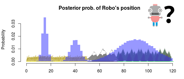
So, this is (in Bayesian lingo) a posterior distribution, the probability of different “states” after having analyzed the available data. Here the “state” is the location of Robo and looking at the posterior above it seems like he could be in a lot of places. Most likely he is in the forest, somewhere between 75 and 120 miles from the reference point (arbitrarily set to the left most position on the map). He might also be hiding in the plains, either around the 15th or the 40th mile. It’s not that likely that he’s in the mountains, but we can’t dismiss it altogether.
- So, where should we start looking for Robo?
- Well, that depends…
- Depends on what?
- Your loss function.
A loss function is some method of calculating how bad a decision would be if the world is in a certain state. In our case the state is the location of Robo, the decision could be where to start looking for him, and badness could be the time it will take to find him (we want to find him fast!). If we knew the state of the world, we could find the best decision: the decision that minimizes the loss. Now, we don’t actually know that state but, if we have a Bayesian model that we believe does a good job, we can use the resulting posterior to represent our knowledge about that state. That is, we are going to plug in a possible decision, and a posterior distribution, to our loss function and the result will be a probability distribution over how large the loss might be. Doing this is really easy, especially if the posterior is represented as a sample of values (which is almost always the case when doing Bayesian data analysis anyway). Of course, we could skip a formal decision analysis and just look at the posterior and make a non-formalized decision. In many case that might be the preferred course, but it’s not why we are here today.
So we call our science team up and ask them to send over the posterior represented as a large sample of positions, let’s call that list s. Here are the first 16 samples in s:
head(s, n = 16)
## [1] 15 101 41 89 14 41 83 112 33 33 94 104 88 82 77 18
As expected, these values are mostly clustered around the 15th, 40th and 90th mile. Say that our loss function is the distance from where we start searching to the location of Robo, and our decision is to start the search at the 60th mile. To get a probability distribution for the loss we simply apply the loss function to each sample in s. For the first sample the loss is abs(15 - 60) = 45, for the second sample it’s abs(101 - 60) = 41, and so on. Below is the resulting posterior loss, given the decision to start searching at the 60th mile:
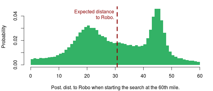
The plot above also show the expected loss (here the mean of the posterior distance from the 60th mile). This is a common measure of how good a decision is and the final step in a decision analysis would be to find the decision that minimizes the expected loss. And that’s it! As Gelman mentioned, the hard part is defining a reasonable loss function, but once you have done that, it’s straight forward to find the decision that minimizes the expected loss.
The rest of the post is dedicated to showing how one can define different loss functions for the “Where’s Robo?” scenario. I will start out with some simple loss functions that result in point estimates and end with some more complicated loss function that result in interval estimates.
What’s the Point?
A Bayesian point estimate is the result of a decision analysis where you (or perhaps your computer) have found the best point/location/value given a posterior distribution and some loss function. Meanwhile, the management have decided that the search party will be deployed by helicopter and that, once on the ground, it will split into two groups, one searching to the right and one searching to the left. Now we only need to decide where to start the search for Robo. Thus, we desperately need a Bayesian point estimate and to get that we need a loss function!
When it comes to loss functions there are three usual suspects: squared loss, absolute loss and 0-1 loss (also known as L2, L1 and L0 loss). We’ve already seen absolute loss (L1), it’s when the loss is the distance between the decision and the state of the world, that is, the absolute value of the difference between the point x and the state s. In R code:
absolute_loss <- function(x, s) {
  mean(abs(x - s))
}
Due to taking the mean, this function will also return the expected absolute loss when s is a posterior sample. For our present purpose this is a pretty decent loss function. Assuming that the two search groups walk at constant speed, this function will minimize the expected time/cost it takes to find Robo.
Squared loss (L2) is another common loss function:
squared_loss <- function(x, s) {
  mean((x - s)^2)
}
Using this loss function would mean that we consider it four times as bad if it takes twice the time to find Robo (again assuming the two search groups walk at constant speed). So squared loss might not make that much sense for the present problem.
The last loss function is 0-1 loss (L0) which assigns zero loss to a decision that is correct and one loss to an incorrect decision. Given this loss function the best decision is to choose the most probable state. This loss function make sense if you are, say, defusing a bomb and need to choose between the green, blue and red wire (if you make the right decision = no loss of limbs, cut the wrong wire = Boom!). When searching for Robo it doesn’t really make sense to say that starting the search 1 mile from Robo’s location is as bad as starting it on the moon. As Robo’s position is a real number, the posterior probability of him being in any specific position is practically zero. In this continuous case we can instead use the posterior probability density. If you have a sample from the posterior (s) then the density can be approximated using density(s). As the resulting density is given at discrete points we have to use approx to interpolate the density at the decision x, and we have to negate the resulting density estimate to turn this into a loss. Here is the whole function:
zero_one_loss <- function(x, s) {
  # This below is proportional to 0-1 loss.
  - approx(density(s), xout = x)$y
}
So, where should we start the search operation according to these three loss functions? To figure this out we just need to determine what decision minimizes the expected loss. This can be done in more or less intelligent ways, but I went brute force and just tried all positions from the 0th to the 120th mile. Here are the resulting point estimates (with the loss functions below):
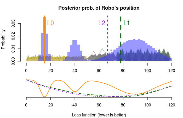
According to the absolute loss criteria (L1) we should start looking in the forest, according to the quadratic loss (L2) we should start in the mountains and 0-1 loss (L0) goes for the single most probable location at the 15th mile. The way with which I found these point estimates is very general, evaluate the loss function all possible decisions (or a representative sample) and pick the decision with the smallest expected loss. However, for these specific loss functions there is a much easier way: the minimum expected absolute loss corresponds to the median of the posterior, the quadratic loss corresponds to the mean, and 0-1 loss corresponds to the mode. That is, the same three point estimates we looked at in Part 1 of Probable Points and Credible Intervals! Why exactly this is the case is beautifully explained by John Myles White on his blog.
Note, that using the three loss functions above result in widely different decisions, it’s a big difference between landing the search team in the forest and in the windy mountains, and it’s a bit strange that the loss functions don’t consider aspects of the problem such as the terrain. Going forward I will explore a couple of different loss functions more suited to the “Where’s Robot?” scenario. This is not because these are loss functions that are especially useful and widely applicable, but rather because I want to show how easy it is to define new loss functions when doing Bayesian decision analysis.
Better Points
We got a call from from management and they have decided that instead of sending a search team, we are going to do a satellite scan that is guaranteed to find any robot within a radius of 30 miles, and now they want to know where to target it. This calls for another loss function! As with 0-1 loss we want to minimize the expectation of not finding Robo, but now it is within a certain radius around the decision point x. In R:
limited_dist_loss <- function(x, s, max_dist) {
  mean(abs(x - s) > max_dist)
}
This code calculates the expectation of Robo being outside the max_dist radius around x, where max_dist should be set to 30 in our case. Using this loss function with our posterior s gives us the following graph:
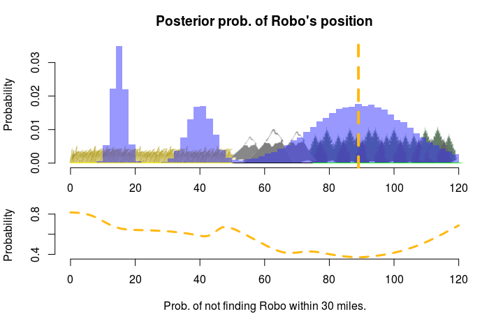
So, we should center the scan on the 89th mile, which will scan the forest and part of the mountains, and which will result in a 1.0 - 0.4 = 0.6 probability of finding Robo.
We got new info from management: The droid carries some space station plans critical to the empire something something. Anyway, we need to find Robo fast, within 24 hours! Again we are going to deploy a search team that will split into two groups, but this time we need to consider how long time it will take for the teams to find him. It takes different amounts of time to search different types of terrain: a mile of plains takes one hour, a mile of forest takes five hours and a mile of mountains takes ten. The list cover_time encodes the time it takes to search each mile, here we have the 48th to the 54th mile:
cover_time[48:54]
##    plain    plain    plain mountain mountain mountain mountain
##        1        1        1       10       10       10       10
The following loss function calculates the expectation of not finding Robo within max_time hours by calculating the time to Robo’s location from the starting point x and then taking the expectation of this time being longer than max_time:
limited_time_loss <- function(x, s, max_time) {
  time_to_robo <- sapply(s, function(robo_pos) {  sum(cover_time[x:robo_pos]) })
  mean(time_to_robo > max_time )
}
This is how the expected loss looks for different starting points with max_time set to 24:
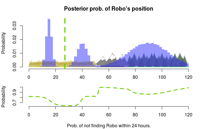
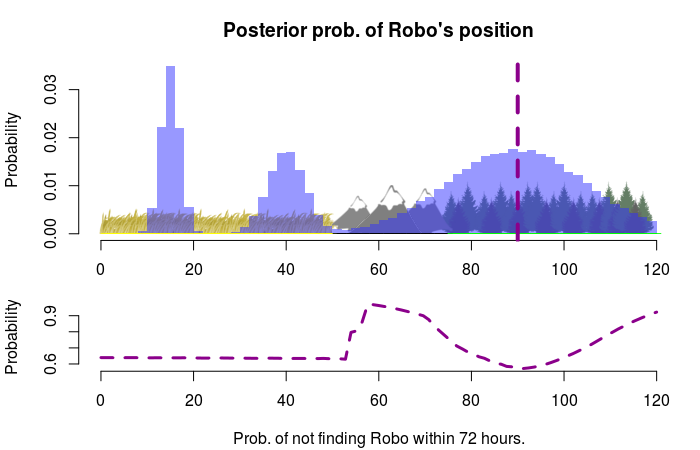
Our best bet is to start at the 27th mile which means we will cover the whole plains area within 24 hours. If we instead had to find Robo within 72 hours it would be better to start at the 90th mile, as we now would have time to search the forest region:
From Points to Intervals
A Bayesian interval estimate is the result of a decision analysis where you have found the best interval given a posterior distribution and some loss function. To decide what interval or region to search through is perhaps a more natural decision when looking for Robo, rather than deciding where to land a search team. In part one we looked at some different type of intervals, one was the highest density interval (HDI) defined as the shortest interval that contains a given percentage of the posterior probability. The HDI can also be defined as the interval that minimizes an expected loss (the specific loss function is derived here, but is a tiny bit complicated). Say that we want to find Robo with 90% probability while having to search through the smallest region. The best decision would then be the following 90% HDI:
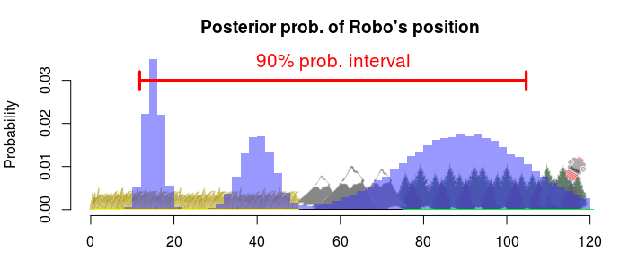
A strange thing with this type of interval is that we limit the probability of finding Robo. Surely we would like to find Robo with the highest probability possible. What’s limiting us from finding Robo with a 100% probability should be time, effort or cost.
Let’s define an interval that is limited by cost instead. The management have decided that the search operation will cost \$1000. One hour of search costs \$100 and using our knowledge about how long time it takes to search a mile of each type of terrain we can calculate the corresponding search cost:
search_cost <- cover_time * 100
search_cost[48:54]
##    plain    plain    plain mountain mountain mountain mountain
##      100      100      100     1000     1000     1000     1000
So searching through the 48th to the 54th mile would cost \$4300, a bit over budget. What we want to find is the interval with the highest expectation of finding Robo but that costs no more than \$1000 to search through. The loss function is basically just a variation of limited_time_loss but with two parameters: the lower and the upper endpoints of the interval. To find the best interval I, again, just try all combinations of upper and lower endpoints and pick out the interval with the lowest loss (highest expectation of finding Robo) which costs \$1000 or less to search through:

So, if we just have \$1000 to spend we should go for the easy option and just search through the high probability region on the plains. What if we had \$3000 to spend?
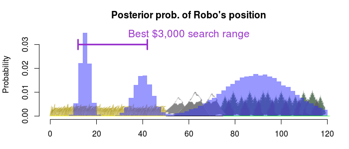
Then we should search through almost the whole plains region. What if we had \$20,000?
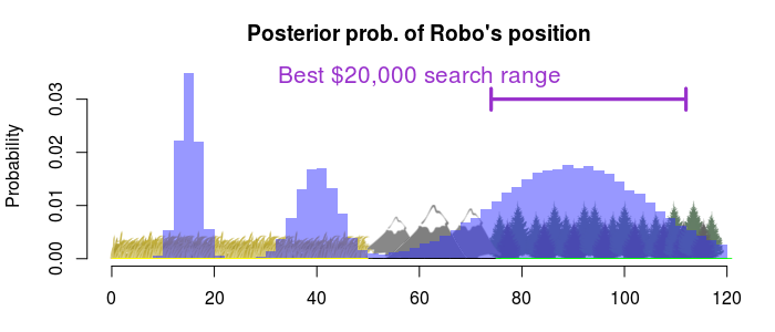
Then we should go for the forest (and still stay away from the mountains, they don’t make good fiscal sense).
Now, we call up management and tell them that “it’s all good and well that you want to spend \$1000 on finding Robo, but why \$1000 exactly? And wouldn’t you want to spend as little as possible?” They tell us that, yes, they would like to spend as little as possible and the reason for the \$1000 figure is because that’s what Robo is worth. Ok, so what we want to do is to mount a search that maximizes the expected profit considering that Robo is worth \$1000 and that it costs \$100 per search hour. This calls for a utility function (something you want to maximize) which is just the opposite of a loss function (something you want to minimize). While any utility function can easily be cast into a loss function, it’s sometimes more natural to think of maximizing utility (say in finance) than minimizing losses. Loss functions and utility functions can both be called objective functions.
This is going to be the most complicated objective function in this post. The search is going to happen like this: We are going to start the search at one location, search in one direction, and stop the search if (1) we find Robo or (2) we have reached the location that marks the end of the search operation. The decision we have to make is where the search starts and where it terminates (in case we don’t find Robo). What we want to calculate is the expected profit given such a decision. The following function takes a start, an end and a robo_value, calculates the profit for each sample from Robo’s posterior position s and returns the expected profit:
expected_profit <- function(start, end, robo_value, s) {
  posterior_profit <- sapply(s, function(robo_pos) {
    if(robo_pos >= start & robo_pos <= end) {
      #that is, we find Robo and terminate the search at robo_pos
      covered_ground <- start:robo_pos
      robo_value - sum(search_cost[covered_ground])
    } else {
      # that is, we won't find Robo and terminate the search at end instead,
      covered_ground <- start:end
      - sum(search_cost[covered_ground])
    }
  })
  mean(posterior_profit)
}
If we evaluate this utility function for (a representative sample of) all possible values for start and end, and with robo_value set to 1000, the maximum expected profit decision is this interval:
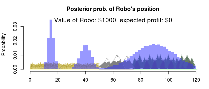
Huh? That doesn’t look like an interval… But it is, you’re looking at an empty interval. The best decision is to not search for Robo at all (with an expected profit of \$0) any search operation will result in an expected negative profit (that is, a loss). Good to know! What if Robo was worth more money? Say, \$10,000?
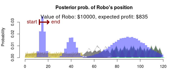
Then we should search a small part of the plains, starting at the 12th mile, for an expected profit of \$835. If Robo was worth \$20,000?
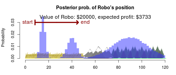
Then we should search most of the plains, still starting from the left, for an expected profit of \$3733. Say, if Robo was really valuable?
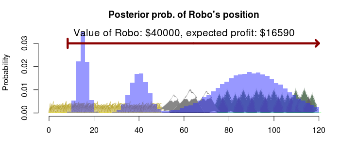
Then we want to search the whole strip of land for an expected profit of \$16590. Notice that we should always start at the left, this is because it is relatively cheap to search the plains and our profit will be much higher if we find Robo before we spend to much on the search operation.
Wrap up
So this was just a sample of possible loss/utility functions for a simple toy problem, some better and some worse. I stuck with point decisions and interval decisions, but there is no reason for why you should be limited to single intervals. Perhaps you want launch several search parties, or perhaps you want to update the decision as you get new information. Constructing reasonable loss functions for real world problems can be very challenging, but the point is that Bayesian decision analysis still works in the same way as outlined in this post: (1) Get a posterior, (2) define a loss function, (3) find the decision that minimizes the expected loss. My toy example featured only a one-dimensional posterior, but the procedure would be no different with a multi-dimensional posterior (except for the added difficulty of optimizing a high-dimensional loss function).
Update: João Pedro at Faculdade de Ciências da Universidade de Lisboa has reimplemented the Robo scenario, but in 2D! Check it out, it’s really nice!
Another point I want to get across is that loss/utility functions are models of what’s bad/good and as such they can be made arbitrarily complex and are in some sense never “true”, in the same way as a statistical model of some process is never the “true” model. Or as Hennig and Kutlukaya (2007) puts it:
“There is no objectively best loss function, because the loss function defines what ‘good’ means.”
By the way, did you find Robo?
References
Hennig, C., & Kutlukaya, M. (2007). Some thoughts about the design of loss functions. REVSTAT–Statistical Journal, 5(1), 19-39. pdf
White, J. M. (2013). Modes, Medians and Means: A Unifying Perspective. link
Berger, J. O. (1985). Statistical decision theory and Bayesian analysis. Springer. Amazon link
Chapter 9 in Gelman et al (2013). Bayesian data analysis. CRC press. Amazon link