Hello stranger, and welcome! 👋😊
I'm Rasmus Bååth, data scientist, engineering manager, father, husband, tinkerer,
tweaker, coffee brewer, tea steeper, and, occasionally, publisher of stuff I find
interesting down below👇
Now that I’ve got my hands on
the source of the cake
dataset I knew I had to attempt to
bake the cake too. Here, the emphasis is on attempt, as there’s no way
I would be able to actually replicate
the elaborate and
cake-scientifically rigorous
recipe that Cook
followed in her thesis. Skipping things like beating the eggs exactly
“125 strokes with a rotary beater” or wrapping the grated chocolate “in
waxed paper, while white wrapping paper was used for the other
ingredients”, here’s my version of Cook’s Recipe C, the highest rated
cake recipe in the thesis:
~~ Frances E. Cook's best chocolate cake ~~

- 112 g butter (at room temperature, not straight from the fridge!)
- 225 g sugar
- ½ teaspoon vanilla, extract or sugar.
- ¼ teaspoon salt
- 96 g eggs, beaten (that would be two small eggs)
- 57 g dark chocolate (regular dark chocolate, not the 85% masochistic kind)
- 122 g milk (that is, ½ a cup)
- 150 g wheat flour
- 2½ teaspoon baking powder

1. In a bowl mix together the butter, sugar, vanilla, and salt
   using a hand or stand mixer.
2. Add the eggs and continue mixing for another minute.
3. Melt the chocolate in a water bath or in a microwave oven.
   Add it to the bowl and mix until it's uniformly incorporated.
4. Add the milk and mix some more.
5. In a separate bowl combine the flour and the baking powder.
   Add it to the batter, while mixing, until it's all combined evenly.
6. To a "standard-sized" cake pan (around 22 cm/9 inches in diameter)
   add a coating of butter and flour to avoid cake stickage.
7. Add the batter to the pan and bake in the middle of the oven
   at 225°C (437°F) for 24 minutes.
Here’s now some notes, photos, and data on how the actual cake bake went
down.
In statistics, there are a number of classic datasets that pop up in examples, tutorials, etc. There’s
the iris dataset (just type iris in your nearest R prompt),
the Palmer penguins (the modern iris alternative),
the titanic dataset(s) (I hope you’re not a guy in 2nd or 3rd class!), etc. While looking for a dataset to illustrate a simple hierarchical model I stumbled upon another one: The cake dataset in
the lme4 package which is described as containing “data on the breakage angle of chocolate cakes made with three different recipes and baked at six different temperatures [as] presented in Cook (1938)”. For me, this raised a lot of questions: Why measure the breakage angle of chocolate cakes? Why was this data collected? And what were the recipes?
I assumed the answers to my questions would be found in Cook (1938) but, after a fair bit of flustered searching, I realized that this scholarly work, despite its obvious relevance to society, was nowhere to be found online. However, I managed to track down that there existed a hard copy at Iowa State University, accessible only to faculty staff.
The tl;dr: After receiving help from several kind people at Iowa State University, I received a scanned version of Frances E. Cook’s Master’s thesis, the source of the cake dataset. Here it is:
Cook, Frances E. (1938). Chocolate cake: I. Optimum baking temperature. (Master’s thesis, Iowa State College).
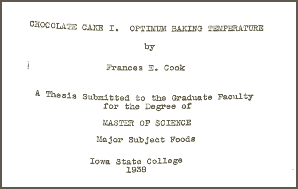
It contains it all, the background, the details, and the cake recipes! Here’s some more details on the cake dataset, how I got help finding its source, and, finally, the cake recipes.
If you know one thing about bubble sort, it’s that it’s a horrible sorting algorithm. But Bubble sort is great for one thing. Bubble sort has one good use case: Beer tasting. Let me explain:
I’ve now been in the industry long enough to know that meetings are often too long. No one likes to be in meetings, and the longer they are, the worse it is. Not only do I know most meetings are too long, but I also know exactly how long a meeting should be, at most! Let’s not delay it any further; here’s Rasmus’s maximum meeting length formula:
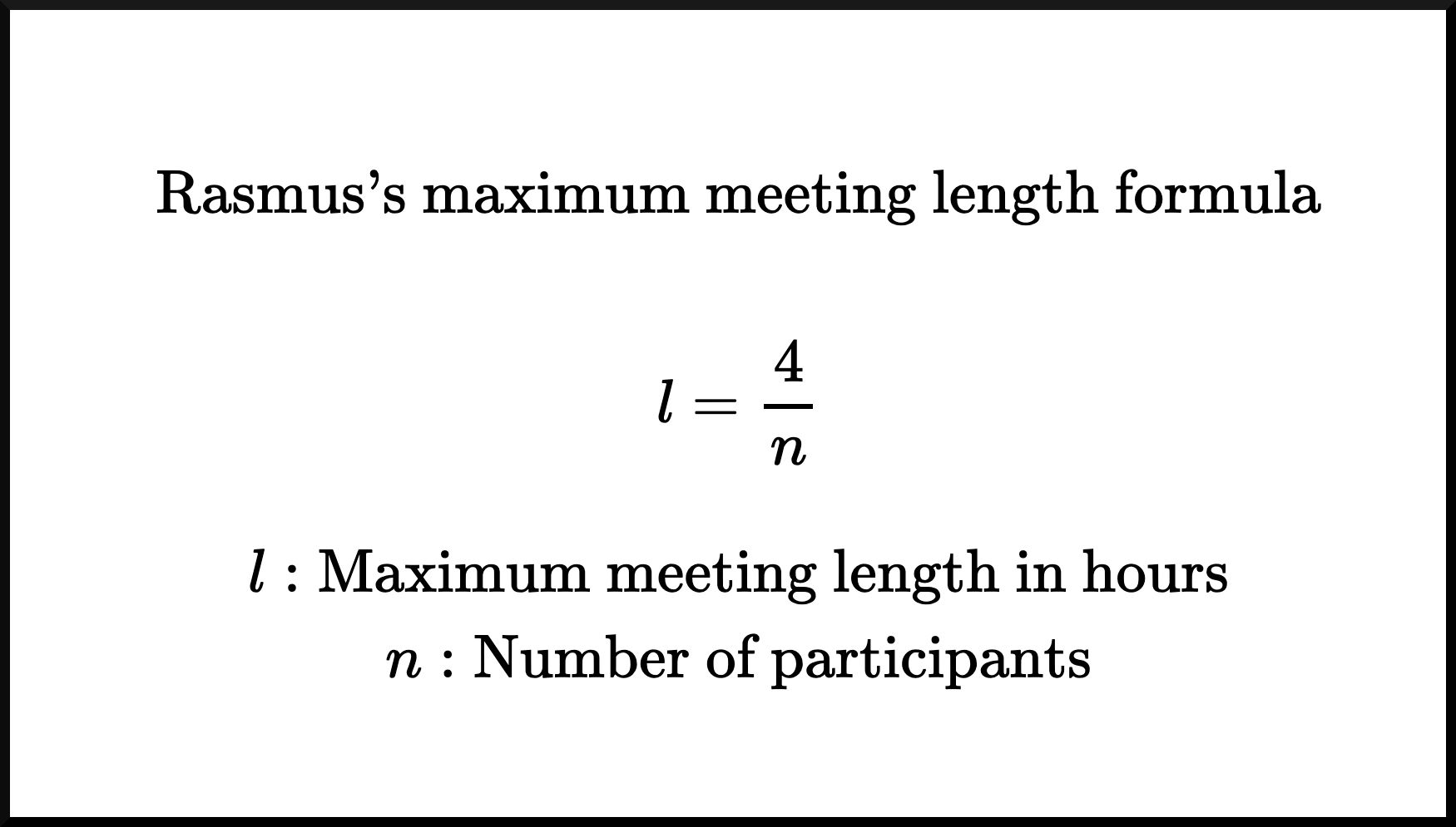
You can see that I’m confident about the correctness of this formula, as I’ve already branded it with my own name and rendered it in $\LaTeX$.
If that’s not enough to convince you, let me break it down further:
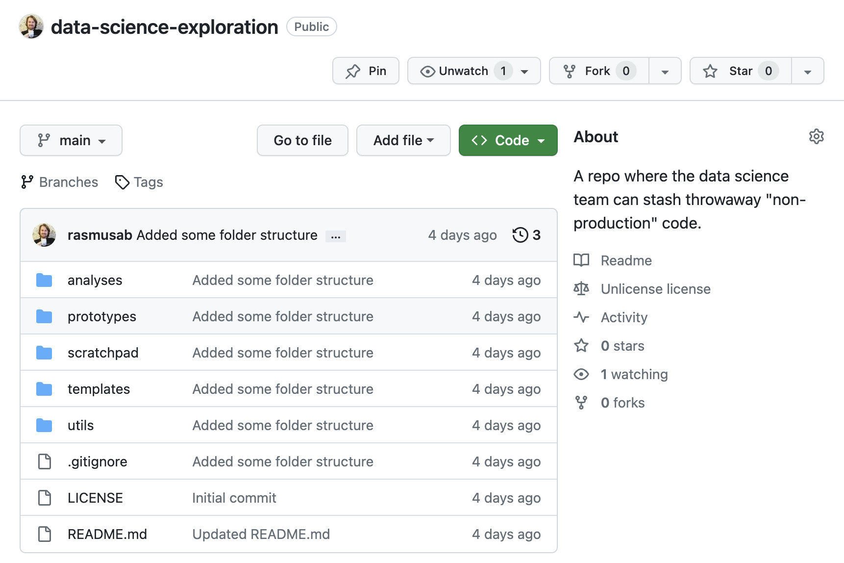
When I started working as a Data Scientist nearly ten years ago, the data science team I joined did something I found really strange at first: They had a single GitHub repo where they put all their “throwaway” code. An R script to produce some plots for a presentation, a Python notebook with a machine learning proof-of-concept, a bash script for cleaning some logs. It all went into the same repo. Initially, this felt sloppy to me, and sure, there are better ways to organize code, but I’ve come to learn that not having a single place for throwaway code in a team is far worse. Without a place for throwaway code, what’s going to happen is:
- Some ambitious person on the team will create a new GitHub repo for every single analysis/POC/thing they do, “swamping” the GitHub namespace.
- Some others will stow their code on the company wiki or drop it in the team Slack channel.
- But most people aren’t going to put it anywhere, and we all know that code “available on request” often isn’t available at all.
So, in all teams I’ve worked in, I’ve set up a GitHub repo that looks something like this:
If you’ve ever looked at a Makefile in a python or R repository chances are that it contained a collection of useful shell commands (make test -> runs all the unit tests, make lint -> runs automatic formatting and linting, etc.). That’s a perfectly good use of make, and if that’s what you’re after then
here’s a good guide for how to set that up. However, the original reason why make was made was to run shell commands, which might depend on other commands being run first, in the right order. In
1976 when Stuart Feldman created make those shell commands were compiling C-programs, but nothing is stopping you from using make to set up simple data pipelines instead. And there are a couple of good reasons why you would want to use make for this purpose:
make is everywhere. Well, maybe not on Windows (but it’s
easy to install), but on Linux and MacOS make comes installed out of the box.make allows you to define pipelines that have multiple steps and complex dependencies (this needs to run before that, but after this, etc.), and figures out what step needs to be rerun and executes them in the correct order.make is language agnostic and allows you to mix pipelines with Python code, Jupyter notebooks, R code, shell scripts, etc.
Here I’ll give you a handy template and some tips for building a data pipeline using python and make. But first, let’s look at an example data pipeline without make.
The first thing I thought when I tried all the cool tools of the Year of the AI Revolution (aka 2022) was: OMG this is amazing, it’s the AI future that I never thought I would see. The second thing I thought was: OMG this is going to be used to spam the internet with so much bland auto-generated content.
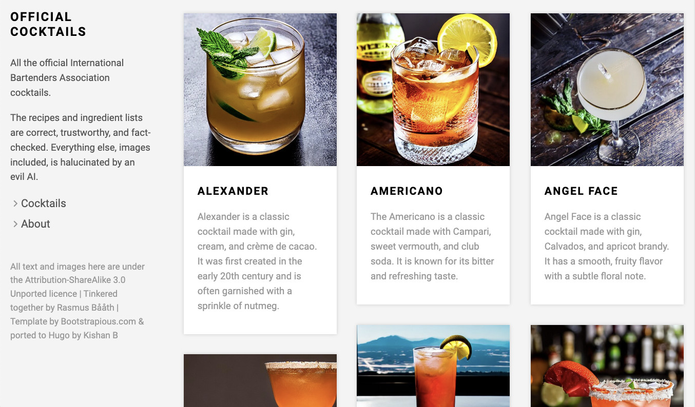
I hate bland auto-generated content as much as the next person, but I was tempted by the forbidden fruit, I irresponsibly took a bite, and two short R scripts and a weekend later I’m now the not-so-proud owner of
officialcocktails.com: A completely auto-generated website with recipes, description, tips, images, etc. covering all the official International Bartenders Association cocktails.
Here’s the quick recipe for how I whipped this up.
Yesterday I put up
a post where I described how I scraped The International Bartenders Association (IBA) cocktails into csv and json format.
Timothy Wolodzko had a reasonable question regarding this on
Mastodon:
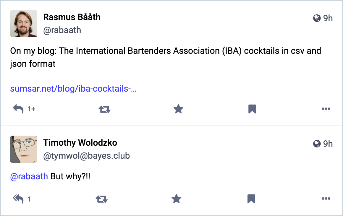
Two reasons:
- Data that’s not sitting in a CSV file make me a bit nervous.
- With data snugly in a CSV file, there are so many things you can do with it! 😁
I find it fascinating that the International Bartenders Association (IBA) keeps a list of “official” cocktails. Like, it’s not like the
World Association of Chefs’ Societies
keeps a list of official dishes. But yet the IBA keeps a list of official cocktails and keeps this up to date (!), as well. For example, I have sad news for all you vodka and orange juice fans out there: As of 2020
the Screwdriver is not an official cocktail anymore.
While a list of official cocktails is a bit silly, it’s also a nice dataset that I’ve now scraped and put into an
iba-cocktails repo. This includes all the International Bartenders Association (IBA) Official Cocktails in CSV and JSON format as of 2023, from two different sources:
The IBA website and
Wikipedia’s list of IBA cocktails. My take on the difference between these sources is that the IBA website is more “official” (it’s their list, after all), but the Wikipedia recipes are easier to follow.
It’s March 2023 and right now
ChatGPT, the amazing AI chatbot tool from OpenAI, is all the rage. But when OpenAI released their public web API for ChatGPT on the 1st of March you might have been a bit disappointed. If you’re an R user, that is. Because, when scrolling through
the release announcement you find that there is a python package to use this new API, but no R package.
I’m here to say: Don’t be disappointed! As long as there is a web API for a service then it’s going to be easy to use this service from R, no specialized package needed. So here’s an example of how to use the new (as of March 2023) ChatGPT API from R. But know that when the next AI API hotness comes out (likely April 2023, or so) then it’s going to be easy to interface with that from R, as well.