In the last post I showed how to use Laplace approximation to quickly (but dirtily) approximate the posterior distribution of a Bayesian model coded in R. This is just a short follow up where I show how to use importance sampling as an easy method to shape up the Laplace approximation in order to approximate the true posterior much better. But first, what is importance sampling?
Importance Sampling
Importance sampling is a method that can be used to estimate the integral of a function even though we only have access to the density of that function at any given point. Using a further resampling step, this method can be used to produce samples that are (approximately) distributed according to the density of the given function. In Bayesian statistics this is what we often want to do with a function that describes the density of the posterior distribution. In the case when there is more than one free parameter the posterior will be multidimensional and there is nothing stopping importance sampling from working in many dimensions. Below I will only visualize the one dimensional case, however.
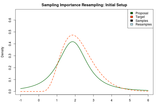
The first step in the importance sampling scheme is to define a proposal distribution that we believe covers most of our target distribution, the distribution that we actually want to estimate. Ideally we would want to choose a proposal distribution that is the same as the target distribution, but if actually could do this we would already be able to sample from the target distribution and importance sampling would be unnecessary. Instead we can make an educated guess. A sloppy guess is to use a uniform proposal distribution that we believe covers most of the density of the target distribution. For example, assuming the target distribution has most of its density in $[-4,4]$ we could setup the importance sampling as:
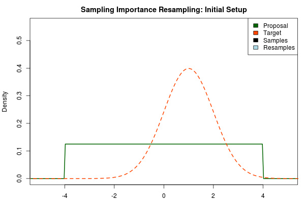
Here, the target distribution is actually a $\text{Normal}(\mu=1,\sigma=1)$ distribution, but most often we do not know its shape.
The next step is to sample from the proposal distribution. For each sample we calculate the likelihood of getting that sample from the target distribution relative to the likelihood of sampling it from the proposal distribution. After we’ve finished sampling we normalize these relative likelihoods so that they sum to one, thus now forming a discrete probability distribution. That is, for each sample $x_i$ we calculate:
$$ p_i = \frac{\text{Target}(x_i) / \text{Proposal}(x_i)}{\sum\nolimits_{x} \text{Target}(x) / \text{Proposal}(x)} $$
where $p_i$ is the final probability of $x_i$ and $\text{Proposal}(\cdot)$ and $\text{Target}(\cdot)$ are the two respective density functions. The resulting discrete probability distribution over all $x_i$ is now an estimate of the target distribution. The procedure is visualized below where the “height” of the samples indicate their respective probability:
We can now use the resulting discrete probability distribution to calculate, for example, the amount of probability above zero by summing all $p_i$ from samples $x_i$ above zero. However, I believe it is easier to work with samples that I can treat as being sampled from the target distribution. With such samples, instead of summing the $p_i$ for samples above zero, I could simply count the number of samples above zero, compare this with the total number of samples and in this way calculate the amount of probability above zero. So as a last step, to get samples that I can treat as being sampled from the target distribution, I (re)sample with replacement from the discrete probability distribution defined by the $x_i\text{s}$ and the corresponding $p_i\text{s}$.
Now, there are two issues that need consideration. First, it might actually be a better idea to resample without replacement. If we are unlucky in the initial sampling phase and draw a sample that is extremely unlikely according to the proposal distribution, but very likely according to the target distribution, this sample will get a huge probability. If we are sampling with replacement the value of that sample might end up dominating the distribution of the resulting resamples. Sampling without replacement is more robust, but on the downside we have to produce far more samples in the first sampling phase than we draw resamples in the resampling phase.
A second issue is that we need to find a good proposal distribution. If the proposal distribution is to wide, most samples will fall outside the high density area of the target distribution. Ideally we would want to choose a proposal distribution that looked similar to the target. If only there was a quick and dirty method that we could use to approximate the distribution of the target density… *cough* *cough* Laplace approximation *cough*
Importance Sampling ❤ Laplace Approximation
Importance Sampling and Laplace Approximation is such a good match! Laplace approximation quickly produces an approximation to the posterior, but it is often a bit off… Importance sampling converges to the true posterior, but this could take (literary) eons if the proposal distribution is very different from the target distribution… Ergo, we use the Laplace approximated posterior as the proposal distribution in importance sampling! With one important modification, however. Below is an importance sampling setup with the Laplace approximation to the posterior distribution as the proposal distribution:
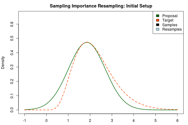
As the target distribution is right skewed the symmetric Laplace approximation is doing a bad job. But using the Laplace approximation as the proposal distribution would currently not really work either. The Laplace approximation is a normal distribution and as such it has very light tails. In an importance sampling scheme we would want the proposal distribution to cover the target distribution but the light tails of the normal distribution make proposal distribution have very low density in areas where the target distribution has a relatively high density (look at the density at 4-5 in the plot above).
The solution is to use a heavy-tailed distribution for the proposal and here a convenient choice is the t-distribution where the degrees-of-freedom parameter decides the fatness of the tails (lower df = fatter tails, when df → $\infty$ the t-distribution approaches the normal distribution). Below, the proposal has been changed to a t-distribution with df = 2 but with the same mean and scale as above.
Being confident that we now have an adequate proposal distribution we can continue with the importance sampling:
Note that in the above animation we sample with replacement but, as argued earlier, it might actually be a good idea to sample without replacement.
So to compare, the true 95% credible interval of the target distribution is $[0.82,4.32]$ but the Laplace approximation gave $[0.20,3.51]$. A final Importance sampling step using 25000 samples and 5000 resamples without replacement yielded $[0.82,4.36]$, which is much closer to the true 95% CI!
Doin’ it in R
Using the function below it is possible to do Laplace approximation of a Bayesian model followed by an optional importance sampling step. The function is designed along the same lines as the one in Easy Laplace Approximation of Bayesian Models in R and requires you to have the coda package and the mvtnorm package installed. The function takes the following arguments:
model, a function that takes a vector of parameters as its first argument and returns the log of the unnormalized posterior density.inits, a vector of reasonable starting values for the parameters given in the same order as in themodel.no_samples, number of samples to draw in the first sampling step.no_resamples, number of resamples in the importance sampling step. If this is set to zero (the default) the importance sampling is skipped andno_samplessamples from the Laplace approximation are returned instead.with replacement, a TRUE/FALSE value that decides whether to resample with or without replacement. If sampling without replacement (the default)no_samplesshould be much larger (maybe ten times) thanno_resamples.df, the degrees-of-freedoms of the t-distribution used if doing the importance sampling step...., all other arguments are passed to themodelfunction.
The function returns the samples (or resamples) as an mcmc object which means that we can use the handy functions from the coda package to inspect the result. Here is now the function importance_laplace_approx (including the helper function log_sum_exp) :
library(coda)
library(mvtnorm)

# A more numerically stable way of calculating log( sum( exp( x ))) Source:
# https://r.789695.n4.nabble.com/logsumexp-function-in-R-td3310119.html
log_sum_exp <- function(x) {
    xmax <- which.max(x)
    log1p(sum(exp(x[-xmax] - x[xmax]))) + x[xmax]
}

# Laplace approximation with optional importance sampling step Note that in
# order to avoid numerical instability all densities are on the log-scale.
importance_laplace_approx <- function(model, inits, no_samples, no_resamples = 0,
    with_replacement = F, df = 2, ...) {
    fit <- optim(inits, model, control = list(fnscale = -1), hessian = TRUE,
        ...)
    param_mean <- fit$par
    param_cov_mat <- solve(-fit$hessian)
    if (no_resamples <= 0) {
        # Just sample from the Laplace distribution
        samples <- rmvnorm(no_samples, param_mean, param_cov_mat)
        return(mcmc(samples))

    } else {
        # Importance sample
        samples <- rmvt(no_samples, delta = param_mean, sigma = param_cov_mat,
            df = df)
        colnames(samples) <- names(inits)
        prop_dens <- dmvt(samples, param_mean, param_cov_mat, df = df)
        target_dens <- apply(samples, 1, model, ...)
        target_dens[!is.finite(target_dens)] <- -Inf
        weighted_dens <- target_dens - prop_dens
        sample_prob <- exp(weighted_dens - log_sum_exp(weighted_dens))
        resample_i <- sample(nrow(samples), size = no_resamples, replace = with_replacement,
            prob = sample_prob)
        resamples <- samples[resample_i, , drop = FALSE]
        colnames(resamples) <- names(inits)
        return(mcmc(resamples))
    }
}
Let’s try it out on the model from Three Ways to Run Bayesian Models in R, that is:
$$y_i \sim \text{Normal}(\mu,\sigma)$$
$$\mu \sim \text{Normal}(0,100)$$
$$\sigma \sim \text{LogNormal}(0,4)$$
where $y$ is 20 datapoints generated like the following:
set.seed(1337)
y <- rnorm(n = 20, mean = 10, sd = 5)
c(mean = mean(y), sd = sd(y))
##   mean     sd
## 12.721  5.762
Here is the corresponding model function calculating the unnormalized log posterior of the model above given a parameter vector p and a vector of datapoints y.
model <- function(p, y) {
    log_lik <- sum(dnorm(y, p["mu"], p["sigma"], log = T))  # the log likelihood
    log_post <- log_lik + dnorm(p["mu"], 0, 100, log = T) + dlnorm(p["sigma"],
        0, 4, log = T)
    log_post
}
First let’s run a Laplace approximation without the resampling step by letting no_resamples = 0 (the default):
samples <- importance_laplace_approx(model, c(mu = 0, sigma = 1), y = y, no_samples = 5000)
densityplot(samples)
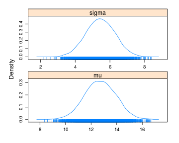
summary(samples)
##
## Iterations = 1:5000
## Thinning interval = 1
## Number of chains = 1
## Sample size per chain = 5000
##
## 1. Empirical mean and standard deviation for each variable,
##    plus standard error of the mean:
##
##        Mean    SD Naive SE Time-series SE
## mu    12.72 1.224   0.0173         0.0173
## sigma  5.45 0.839   0.0119         0.0119
##
## 2. Quantiles for each variable:
##
##        2.5%   25%   50%   75% 97.5%
## mu    10.33 11.88 12.72 13.57  15.1
## sigma  3.81  4.88  5.45  6.02   7.1
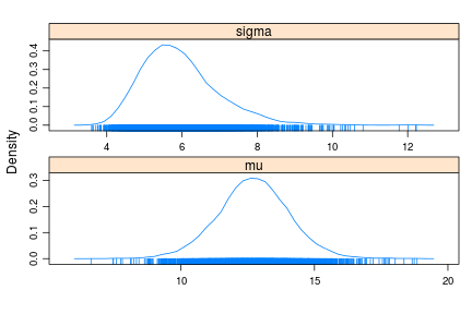
Here the 95% CI for sigma is $[3.81,7.10]$ which is a bit off compared to the actual 95% posterior CI which is $[4.38,8.39]$. Now, let’s see if we can improve on that by running the extra importance sampling step by setting no_resamples = 5000 and increasing no_samples to 25000.
samples <- importance_laplace_approx(model, c(mu = 0, sigma = 1), y = y, no_samples = 25000,
    no_resamples = 5000)
## There were 50 or more warnings (use warnings() to see the first 50)
Hmmm, why the warnings? Well, the importance sampling step does not honor the boundaries of the parameters in our model and regularly tries sigmas that are negative resulting in NaN. We could fix this by checking if the parameters are within the bounds in the model function and if not return -Inf or we could happily ignore these warnings as importance_laplace_approx sets all NaNs to -Inf. So, did the importance sampling improve upon the estimated posterior?
densityplot(samples)
summary(samples)
##
## Iterations = 1:5000
## Thinning interval = 1
## Number of chains = 1
## Sample size per chain = 5000
##
## 1. Empirical mean and standard deviation for each variable,
##    plus standard error of the mean:
##
##        Mean   SD Naive SE Time-series SE
## mu    12.71 1.36   0.0192         0.0192
## sigma  5.95 1.03   0.0146         0.0152
##
## 2. Quantiles for each variable:
##
##        2.5%   25%   50%   75% 97.5%
## mu    10.04 11.87 12.71 13.57 15.40
## sigma  4.36  5.23  5.81  6.49  8.32
Now the posterior of sigma correctly appears right skewed and the 95% CI is $[4.36,8.33]$, much closer to the actual CI.
So, all in all, I believe importance_laplace_approx is a really neat function. You can start off by quickly estimating your model using regular Laplace approximation and then add the importance sampling step when you want to shape up the Laplace approximation.
Disclaimer: I have not tested the function extensively so use it with a pinch of caution. Please tell me if you find an error in it!
I would like to thank Tal Galili for syndicating me on Rbloggers and Yihui Xie for the animation package with which the animations in this post were made.