Thank you for tuning in! In this post, a continuation of Three Ways to Run Bayesian Models in R, I will:
- Handwave an explanation of the Laplace Approximation, a fast and (hopefully not too) dirty method to approximate the posterior of a Bayesian model.
- Show that it is super easy to do Laplace approximation in R, basically four lines of code.
- Put together a small function that makes it even easier, if you just want this, scroll down to the bottom of the post.
But first a picture of the man himself:

Laplace Approximation of Posterior Distributions
Have you noticed that posterior distributions often are heap shaped and symmetric? What other thing, that statisticians love, is heap shaped and symmetric? The normal distribution of course! Turns out that, under most conditions, the posterior is asymptotically normally distributed as the number of data points goes to $\infty$. Hopefully we would then not be too off if we approximated the posterior using a (possibly multivariate) normal distribution. Laplace approximation is a method that does exactly this by first locating the mode of the posterior, taking this as the mean of the normal approximation, and then calculating the variance of the normal by “looking at” the curvature of of the posterior at the mode. That was the handwaving, if you want math, check wikipedia.
So, how well does Laplace Approximation work in practice? For complex models resulting in multimodal posteriors it will obviously not be a good approximation, but for simple models like the generalized linear model, especially when assuming the usual suspects, it works pretty well. But why use an approximation that might be slightly misleading instead of using Markov chain Monte Carlo, an approximation that converges to the true posterior? Well, because Laplace Approximation only has to find the mode of the posterior, it does not have to explore the whole posterior distribution and therefore it can be really fast! I’m talking seconds, not minutes…
Let’s see how well Laplace approximation performs in a couple of simple examples. In the following the the true posterior will be in green and the Laplace approximation will be dashed and red. First up is the posterior for the rate parameter $\theta$ of a Binomial distribution given 10 heads and 8 tails, assuming a flat prior on $\theta$.
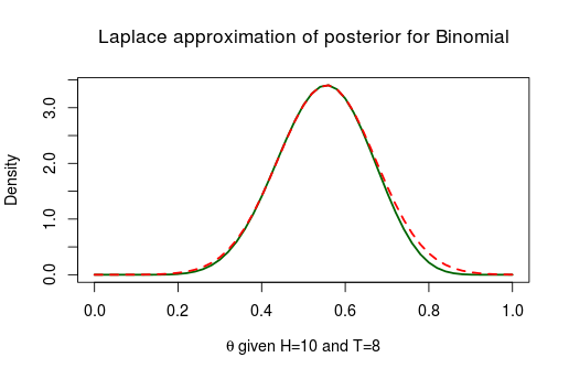
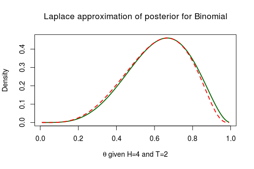
Here the Laplace approximation works pretty well! Now let’s look at the posterior of the same model but with less data, only 4 heads and 2 tails.
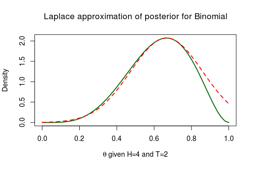
Not working well at all. As the true posterior is slanted to the right the symmetric normal distribution can’t possibly match it. This type of problem generally occurs when you have parameters with boundaries. This was the case with $\theta$ which is bounded between $[0,1]$ and similarly we should expect troubles when approximating the posterior of scale parameters bounded between $[0,\infty]$. Below is the posterior of the standard deviation $\sigma$ when assuming a normal distribution with a fixed $\mu=10$ and flat priors, given 8 random numbers distributed as Normal(10, 4):
rnorm(n = 8, mean = 10, sd = 4)
## [1] 10.770 4.213 8.707 16.489 7.244 18.168 13.775 18.328
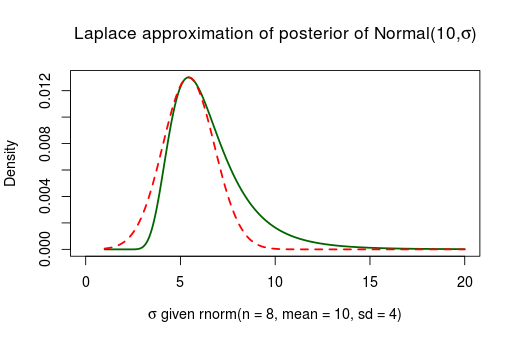
As we feared, the Laplace approximation is again doing a bad job. There are two ways of getting around this, (1) we could collect more data. The more data the better the Laplace approximation will be as the posterior is asymptotically normally distributed. Below is the same model but given 48 data points instead of 8.
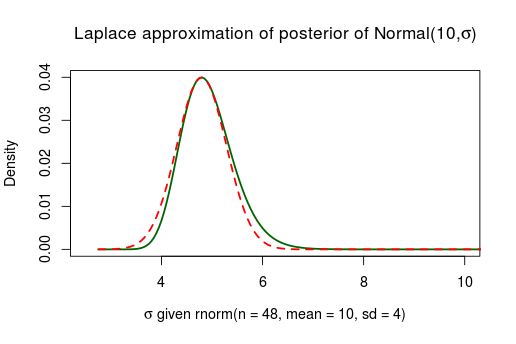
This works better, but to collect more data just to make an approximation better is perhaps not really useful advice. A better route is to (2) reparameterize the bounded parameters using logarithms so that they stretch the real line $[-\infty,\infty]$. An extra bonus with this approach is that the resulting approximation won’t put posterior probability on impossible parameter values such as $\sigma = -1$. Here is the same posterior as above, using the 8 datapoints, the only difference being that the approximation is made on the $\log(\sigma)$ scale.
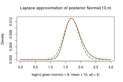
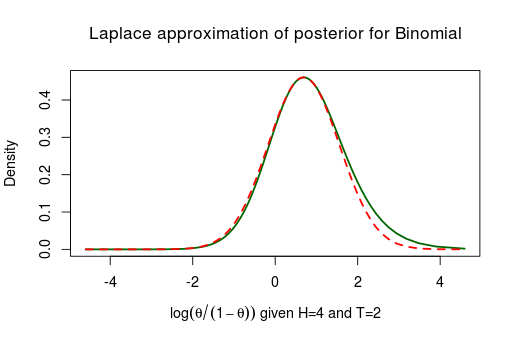
Much better! Similarly we can reparameterize $\theta$ from the binomial model above using the logit transform $\log(\frac{\theta}{1-\theta})$ thus “stretching” $\theta$ from $[0,1]$ onto $[-\infty,\infty]$. Again, now Laplace approximation works much better:
After we have fitted the model using Laplace approximation we can of course transform the the approximated posterior back to the original parameter scale:
Laplace Approximation in R
Seeing how well Laplace approximation works in the simple cases above we are, of course, anxious to try it out using R. Turns out, no surprise perhaps, that it is pretty easy to do. The model I will be estimating is the same as in my post Three Ways to Run Bayesian Models in R, that is:
$$y_i \sim \text{Normal}(\mu,\sigma)$$
$$\mu \sim \text{Normal}(0,100)$$
$$\sigma \sim \text{LogNormal}(0,4)$$
Here $y$ is 20 datapoints generated like the following:
set.seed(1337)
y <- rnorm(n = 20, mean = 10, sd = 5)
c(mean = mean(y), sd = sd(y))
##   mean     sd
## 12.721  5.762
First I define a function calculating the unnormalized log posterior of the model above given a parameter vector p and a vector of datapoints y.
model <- function(p, y) {
    log_lik <- sum(dnorm(y, p["mu"], p["sigma"], log = T))  # the log likelihood
    log_post <- log_lik + dnorm(p["mu"], 0, 100, log = T) + dlnorm(p["sigma"],
        0, 4, log = T)
    log_post
}
Here I should probably have reparameterized sigma to not be left bounded at 0, but I’m also a bit curious about how bad the approximation will be when using the “naive” parameterization… Then I’ll find the mode of the two-dimensional posterior using the optim function. As optim performs a search for the maximum in the parameter space it requires a reasonable starting point here given as the inits vector.
inits <- c(mu = 0, sigma = 1)
fit <- optim(inits, model, control = list(fnscale = -1), hessian = TRUE, y = y)
The reason why we set control = list(fnscale = -1) is because the standard behavior of optim is to minimize rather than maximize, setting fnscale to -1 fixes this. The reason why we set hessian = TRUE is because we want optim to return not only the maximum but also the
Hessian matrix which describes the curvature of the function at the maximum.
Now we pick out the found maximum (fit$par) as the mode of the posterior, and thus the mean of the multivariate normal approximation to the posterior. We then calculate the inverse of the negative Hessian matrix which will give us the variance and co-variance of our multivariate normal. For full disclosure I must admit that I have not full grokked why inverting the negative Hessian results in the co-variance matrix, but that won’t stop me, this is how you do it:
param_mean <- fit$par
param_cov_mat <- solve(-fit$hessian)
round(param_mean, 2)
##    mu sigma
## 12.71  5.46
round(param_cov_mat, 3)
##           mu  sigma
## mu     1.493 -0.001
## sigma -0.001  0.705
Now we have all the info we need and we could look at the approximated posterior distribution. But as a last step, I’ll draw lots of samples from the multivariate normal:
library(mvtnorm)
samples <- rmvnorm(10000, param_mean, param_cov_mat)
“Why?”, you may ask, “Why add another layer of approximation?”. Because it takes just a couple of ms to generate 10000+ samples and samples are so very convenient to work with! For example, if I want to look at the posterior predictive distribution (that is, the distribution of a new datapoint given the data) it is easy to add to my matrix of samples:
samples <- cbind(samples, pred = rnorm(n = nrow(samples), samples[, "mu"], samples[,
    "sigma"]))
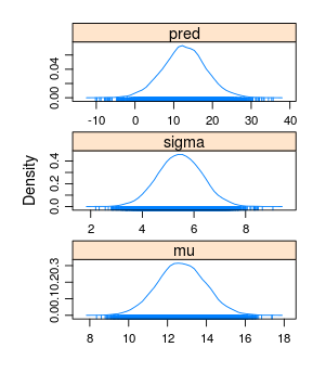
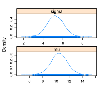
By converting the matrix of samples to an mcmc object I can use many of the handy functions in the coda package to inspect the posterior.
library(coda)
samples <- mcmc(samples)
densityplot(samples)
summary(samples)
##
## Iterations = 1:10000
## Thinning interval = 1
## Number of chains = 1
## Sample size per chain = 10000
##
## 1. Empirical mean and standard deviation for each variable,
##    plus standard error of the mean:
##
##        Mean    SD Naive SE Time-series SE
## mu    12.71 1.225  0.01225        0.01225
## sigma  5.46 0.846  0.00846        0.00762
## pred  12.71 5.655  0.05655        0.05655
##
## 2. Quantiles for each variable:
##
##        2.5%   25%   50%   75% 97.5%
## mu    10.32 11.88 12.70 13.54 15.13
## sigma  3.81  4.89  5.46  6.04  7.13
## pred   1.38  9.01 12.70 16.39 24.05
Now we can compare the the quantiles of the Laplace approximated posterior with the “real” quantiles calculated using JAGS in Three Ways to Run Bayesian Models in R.
##        2.5%   25%   50%   75% 97.5%
## mu    10.03 11.83 12.72 13.60 15.40
## sigma  4.38  5.27  5.86  6.57  8.39
The Laplace approximation of mu was pretty spot on while the approximation for sigma was a little bit off as expected (it would have been much better if we would have reparameterized sigma). Note that many of the coda functions also produce MCMC diagnostics that are not applicable in our case, for example Time-series SE above.
At Last, a Handy Function
Let’s wrap up everything, optimization and sampling, into a handy laplace_approx function.
library(coda)
library(mvtnorm)

# Laplace approximation
laplace_approx <- function(model, inits, no_samples, ...) {
    fit <- optim(inits, model, control = list(fnscale = -1), hessian = TRUE,
        ...)
    param_mean <- fit$par
    param_cov_mat <- solve(-fit$hessian)
    mcmc(rmvnorm(no_samples, param_mean, param_cov_mat))
}
Here is how to run the same analysis as above using this function.
y <- rnorm(n = 20, mean = 10, sd = 5)

model <- function(p, y) {
    log_lik <- sum(dnorm(y, p["mu"], p["sigma"], log = T))
    log_post <- log_lik + dnorm(p["mu"], 0, 100, log = T) + dlnorm(p["sigma"],
        0, 4, log = T)
    log_post
}

inits <- c(mu = 0, sigma = 1)
samples <- laplace_approx(model, inits, 10000, y = y)
densityplot(samples)
summary(samples)
##
## Iterations = 1:10000
## Thinning interval = 1
## Number of chains = 1
## Sample size per chain = 10000
##
## 1. Empirical mean and standard deviation for each variable,
##    plus standard error of the mean:
##
##        Mean    SD Naive SE Time-series SE
## mu    10.48 1.189  0.01189        0.01189
## sigma  5.26 0.809  0.00809        0.00833
##
## 2. Quantiles for each variable:
##
##       2.5%  25%   50%   75% 97.5%
## mu    8.14 9.69 10.48 11.28 12.82
## sigma 3.69 4.71  5.24  5.81  6.84