There are tons of well-known global indicators. We’ve all heard of gross domestic product, life expectancy, rate of literacy, etc. But, ever since I discovered pinballmap.com, possibly the world’s most comprehensive database of public pinball locations, I’ve been thinking about a potential new global indicator: Public Pinball Machines per Capita. Thanks to Pinball Map’s well-documented public API, this indicator is now a reality!
 Here’s how this was
put together (and just scroll to the bottom for a CSV file with this
indicator for all countries).
Here’s how this was
put together (and just scroll to the bottom for a CSV file with this
indicator for all countries).
Pulling public pinball locations from Pinball Map
Pinball Map is, from what I can discern, the most popular app for finding out where there are arcades and bars with pinball machines. It’s open for anyone to register new pinball locations, but not only that, the app itself is open source, and the data it collects is available through a public API under a permissive licence! Using this API, we will pull essential data for our Public Pinball Machines per Capita indicator: all registered pinball locations and their respective machine counts.
Loading packages
library(httr2) # To interact with the Pinball Map API
library(jsonlite) # To parse the JSON responses
library(tidyverse) # To munch, crunch, and plot the data
library(ggrepel) # For less crowed labels on plots
library(WDI) # To pull in other country-level data
library(maps) # For plotting maps
Code for pulling pinball stats from the Pinball Map API
# We're going to pull a lot of data here, possibly abusing the Pinball Map API,
# a bit. But I'm an active patreon sponsor, so hopefully that's OK...
# Did I mention that they are on patreon? https://www.patreon.com/pinballmap

# Pulls and parses JSON from the given URL
get_req_json <- \(url) {
  request(url)  |>
    req_perform() |>
    resp_body_json(simplifyVector = TRUE)
}

# Pulling all regions defined by the Pinball Map API
regions <- get_req_json("https://pinballmap.com/api/v1/regions.json")$regions

# Now looping over the region names and for each name pull down all locations
region_locations <- lapply(regions$name, \(name) {
  url <- paste0("https://pinballmap.com/api/v1/region/", name, "/locations.json")
  get_req_json(url)$locations
})

# Pull down all "regionless" locations. Actually, most locations are regionless.
regionless_locations <- get_req_json(
  "https://pinballmap.com/api/v1/locations.json?regionless_only=true"
)$locations

# Finally, combine it all...
locations <- bind_rows(region_locations, regionless_locations) |>
  select(name, country, city, lat, lon, num_machines) |>
  mutate(lat = as.numeric(lat), lon = as.numeric(lon)) |>
  # ... and order locations from north to south
  arrange(desc(lat))

sample_n(locations, size = 5)
                        name country          city  lat    lon num_machines
1 Arena Lanes Bowling Center      US      Oak Lawn 41.7  -87.7            3
2              Pete's Treats      US Union Springs 42.9  -76.7            1
3         The Summit Windsor      US      Loveland 40.4 -105.0            6
4             Skylark Lounge      US        Denver 39.7 -105.0            2
5         The Escape Gamebar      US       Atlanta 33.9  -84.3            5
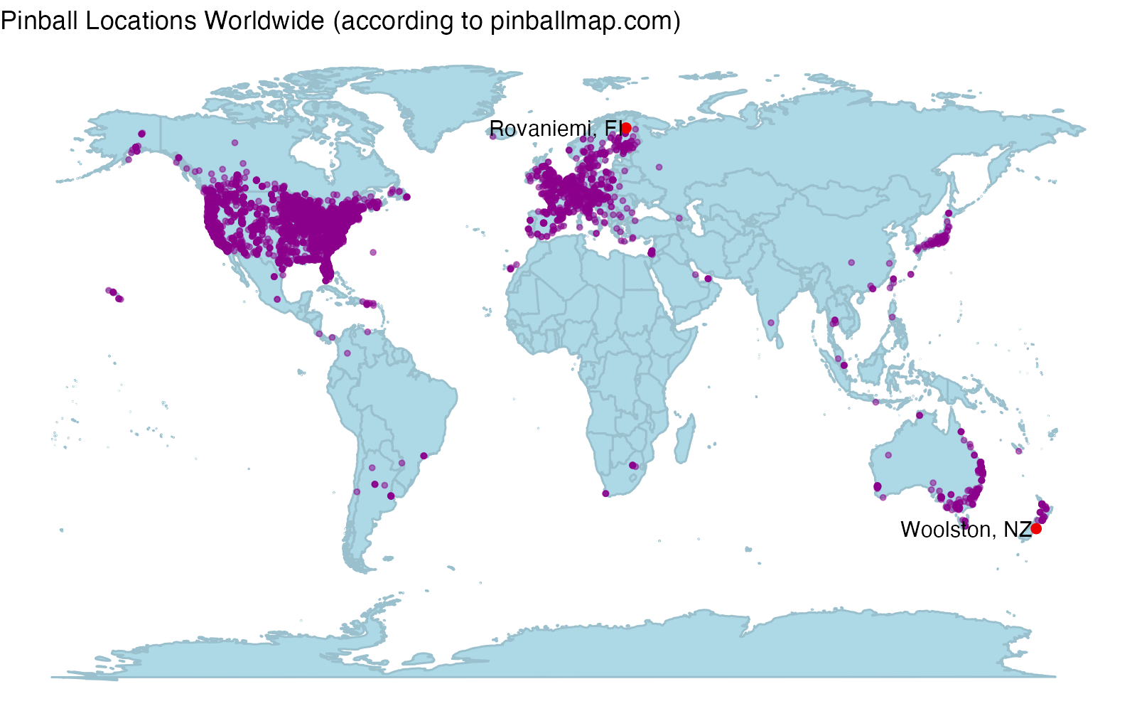
The above shows a sample of five out of the 10,330 locations where you can play pinball, as of June 2024. As we have the longitude and latitude we can also figure out that the northernmost place to play pinball is in Rovaniemi, Finland, and the southernmost place is in Woolston, New Zealand.
Code
locations[c(1, nrow(locations)),]
                       name country      city   lat   lon num_machines
1               Kauppayhtiö      FI Rovaniemi  66.5  25.7            2
10330 Fish & Chips On Ferry      NZ  Woolston -43.5 172.7            1
Or, why not just plot all pinball locations on a world map?
Plot code
extreme_locations <- locations |>
  filter(lat %in% range(lat)) |>
  mutate(display_label = paste(city, country, sep = ", "))

ggplot() +
  geom_polygon(data = map_data("world"), aes(x = long, y = lat, group = group), fill = "lightblue", color = "lightblue3") +
  geom_point(data = locations, aes(x = lon, y = lat), color = "magenta4", size = 1, alpha = 0.50) +
  geom_point(data = extreme_locations, aes(x = lon, y = lat), color = "red2", size = 2) +
  geom_text(data = extreme_locations, aes(x = lon, y = lat, label = display_label), nudge_x = -25) +
  theme_void() +
  ggtitle("Pinball Locations Worldwide (according to pinballmap.com)")
Finally, we can now sum up how many public pinball machines there are in each country, where the USA, unsurprisingly, takes the lead.
Code
pinball_stats <- locations |>
  group_by(country) |>
  summarise(
    n_locations = n(),
    n_machines = sum(num_machines)) |>
  arrange(desc(n_machines))
pinball_stats
# A tibble: 65 × 3
   country n_locations n_machines
   <chr>         <int>      <int>
 1 US             7831      32287
 2 CA              511       1765
 3 AU              427       1247
 4 DE              129       1099
 5 FR              247        707
 6 SE               79        692
 7 GB              160        500
 8 FI               98        496
 9 NL               69        461
10 JP               86        351
# ℹ 55 more rows
Calculating Public Pinball Machines per Capita
Knowing how many public pinball machines there are in each country isn’t
enough, we also need to consider the size of the population. Thanks to
the WDI package it’s easy to
pull this, and any other indicators you fancy, from
the World Bank Open
Data and to calculate the number of Public
Pinball Machines per Capita (here per million people).
Code for pulling World Development Indicators
country_stats_by_year = WDI(
  indicator = c(
    "NY.GDP.PCAP.CD", "SP.POP.TOTL", "SP.DYN.LE00.IN",
    "SP.DYN.TFRT.IN", "IT.NET.USER.ZS", "AG.LND.FRST.ZS"
  ),
  extra = TRUE,
  latest = 1
)

country_stats <- country_stats_by_year |>
  arrange(country, year) |>
  group_by(country) |>
  # Keep the latest indicator for each country
  summarize(across(everything(), \(x) last(na.omit(x)))) |>
  select(
    country_name = country,
    country_code = iso2c,
    gdp_per_capita = NY.GDP.PCAP.CD,
    population = SP.POP.TOTL,
    life_expectancy = SP.DYN.LE00.IN,
    births_per_woman = SP.DYN.TFRT.IN,
    internet_usage_perc = IT.NET.USER.ZS,
    forest_coverage_perc = AG.LND.FRST.ZS
  )
Code for calculating Public Pinball Machines per Capita
pinball_country_stats <- country_stats |>
  # Let's keep only larger countries
  filter(population > 500000) |>
  inner_join(pinball_stats, by = join_by(country_code == country)) |>
  mutate(
    n_locations_per_million_capita = round(n_locations / population * 1000000, 3),
    n_machines_per_million_capita = round(n_machines / population * 1000000, 3)) |>
  arrange(desc(n_machines_per_million_capita))

select(pinball_country_stats,
  country_name, population, n_machines, n_machines_per_million_capita
)
# A tibble: 58 × 4
   country_name  population n_machines n_machines_per_million_capita
   <chr>              <dbl>      <int>                         <dbl>
 1 United States  333287557      32287                          96.9
 2 Finland          5556106        496                          89.3
 3 Sweden          10486941        692                          66.0
 4 Denmark          5903037        323                          54.7
 5 Norway           5457127        266                          48.7
 6 Australia       26005540       1247                          48.0
 7 Canada          38929902       1765                          45.3
 8 New Zealand      5124100        171                          33.4
 9 Switzerland      8775760        267                          30.4
10 Netherlands     17700982        461                          26.0
# ℹ 48 more rows
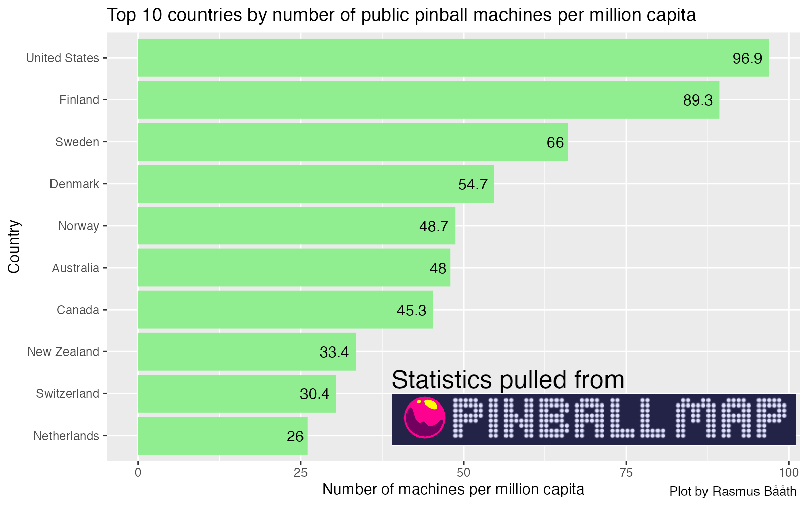
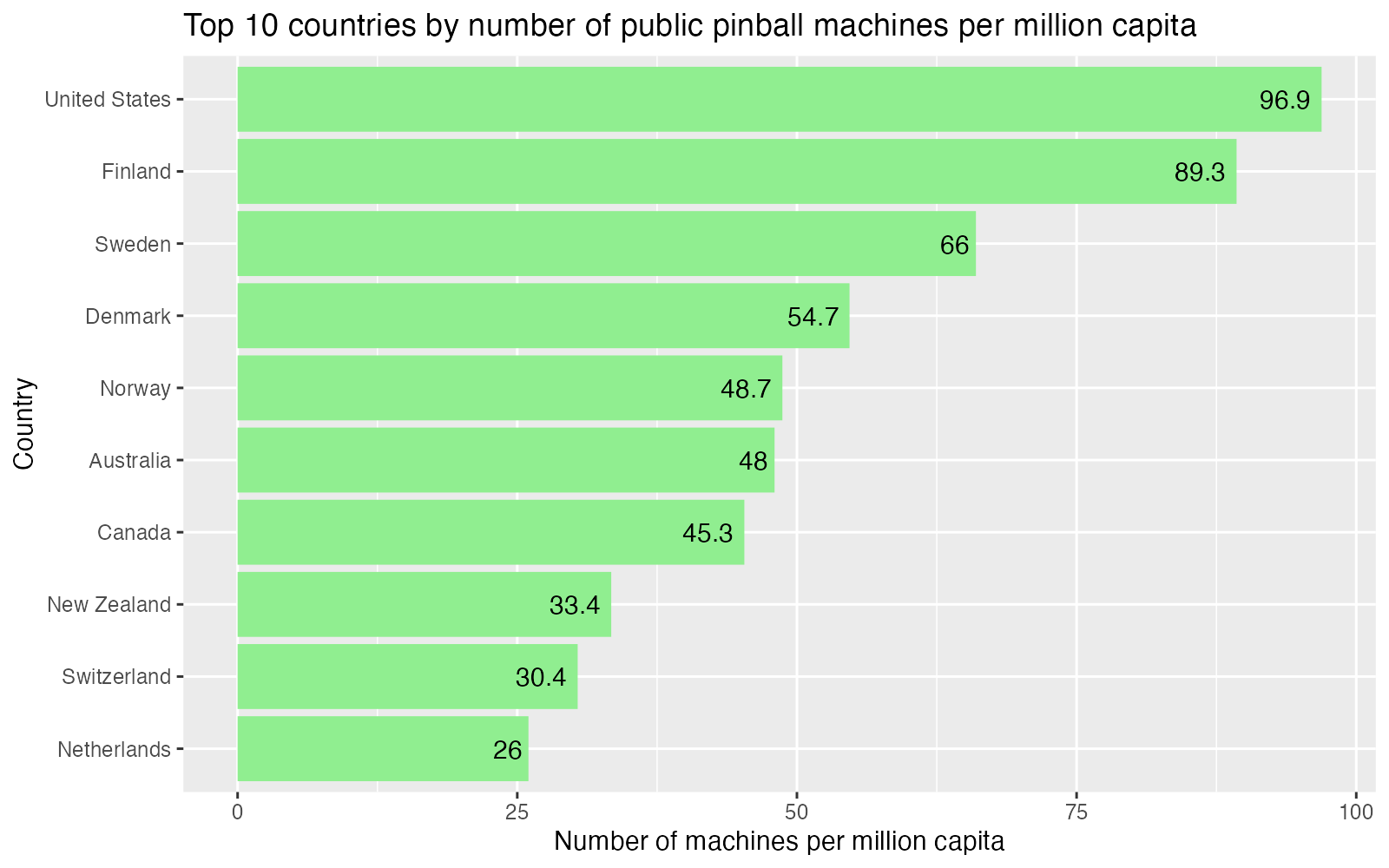
Now, there’s out new global indicator! Looks like the USA is still in the lead, but now the Nordic countries have bubbled up as some of the countries with the highest pinball density.
Plot code
pinball_country_stats |>
  head(10) |>
  mutate(
    country_name = forcats::fct_reorder(country_name, n_machines_per_million_capita),
    n_machines_per_million_capita = round(n_machines_per_million_capita, 1)
  ) |>
  ggplot(aes(x = n_machines_per_million_capita, y = country_name)) +
    geom_col(fill = "lightgreen") +
    geom_text(aes(label = n_machines_per_million_capita), hjust = 1.2) +
    labs(
      x = "Number of machines per million capita",
      y = "Country",
      title = "Top 10 countries by number of public pinball machines per million capita"
    )
Public Pinball Machines per Capita VS other indicators
Let’s have a look at how Public Pinball Machines per Capita compares to some other indicators. How about Life Expectancy?
Plot code
ggplot(pinball_country_stats, aes(x = life_expectancy, y = n_machines_per_million_capita)) +
  geom_label_repel(aes(label = country_name), fill = "lightblue",  max.overlaps = Inf, box.padding  = -0.2) +
  scale_x_log10(labels = scales::label_comma(), limits = c(67, NA)) +
  scale_y_log10(labels = scales::label_comma()) +
  labs(
    x = "Life expectancy at birth (years)",
    y = "Number of machines per million capita",
    title = "Number of Public Pinball Machines per Capita vs life expectancy"
  )
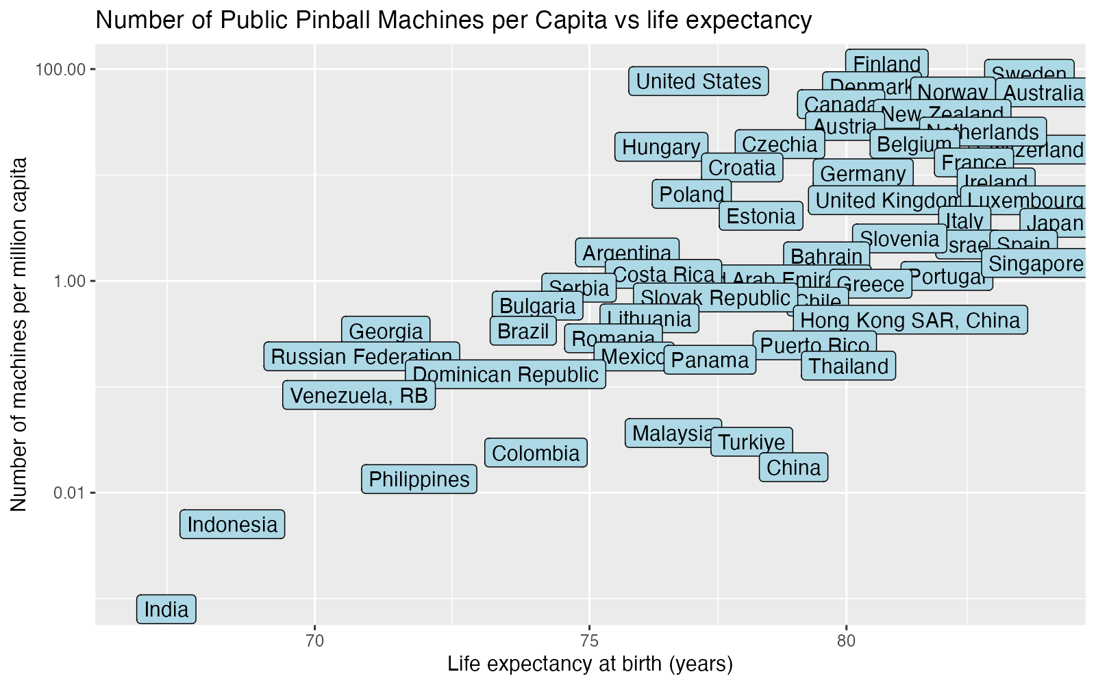
So maybe playing pinball actually makes you live longer! What’s that thing they say about correlation, now again… Or what about the fertility rate (the average number of births per woman)?
Plot code
ggplot(pinball_country_stats, aes(x = births_per_woman, y = n_machines_per_million_capita)) +
  geom_label_repel(aes(label = country_name), fill = "lightcoral",  max.overlaps = Inf, box.padding = -0.2) +
  scale_x_log10(labels = scales::label_comma()) +
  scale_y_log10(labels = scales::label_comma()) +
  labs(
    x = "Fertility rate (no. births per woman)",
    y = "Number of machines per million capita",
    title = "Number of Public Pinball Machines per Capita vs fertility rate"
  )
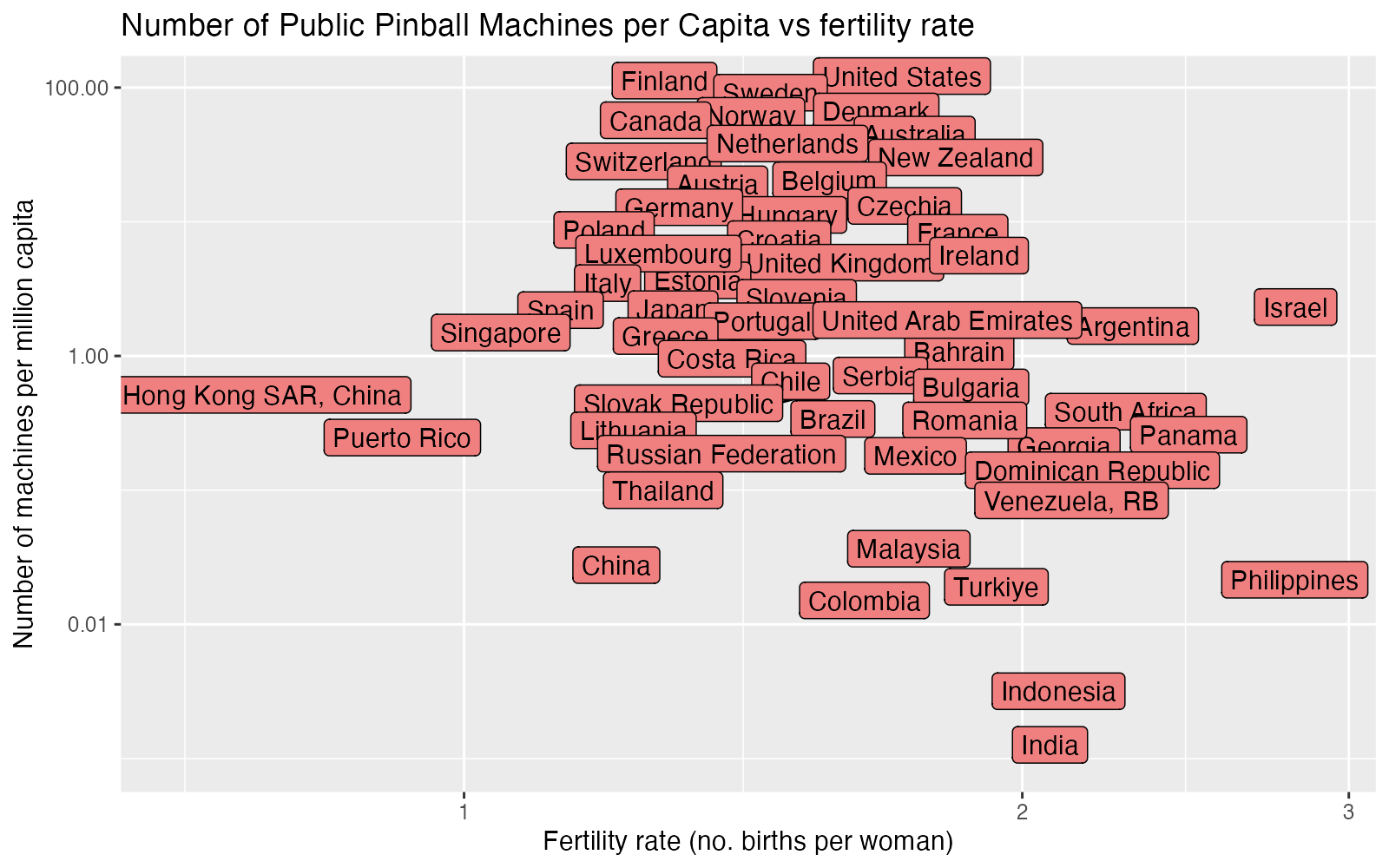
Nope, no clear relationship there. Actually, out of all the indicators I looked through, the one with the highest correlation to Public Pinball Machines per Capita was…
Plot code
ggplot(pinball_country_stats, aes(x = gdp_per_capita, y = n_machines_per_million_capita)) +
  geom_label_repel(aes(label = country_name), fill = "lightgreen", max.overlaps = Inf, box.padding  = -0.2) +
  geom_smooth(method = "lm", se = FALSE, color = "#d03030aa") +
  scale_x_log10(labels = scales::label_comma()) +
  scale_y_log10(labels = scales::label_comma()) +
  labs(
    x = "GDP per capita (in USD)",
    y = "Number of machines per million capita",
    title = "Number of Public Pinball Machines per Capita vs GDP per Capita"
  )
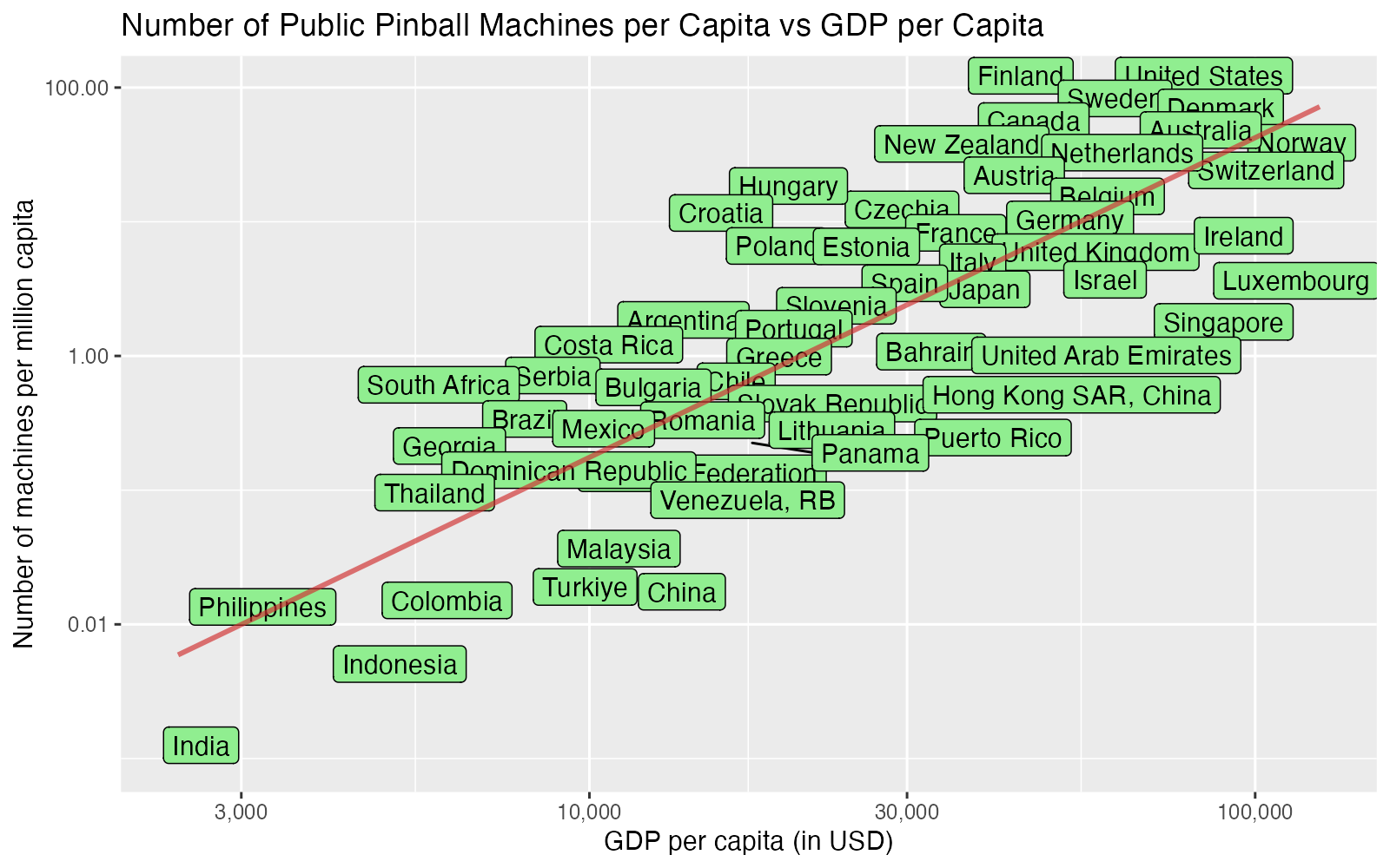
… GDP per Capita. This shouldn’t surprise anyone who’s ever looked into buying a pinball machine and walked away in shock having learned that a new machine would set you back $8000, at least. Still, the correlation between these two indicators is strikingly high:
Code
cor(
  log(pinball_country_stats$n_machines_per_million_capita),
  log(pinball_country_stats$gdp_per_capita)
)
[1] 0.815
With such a strong correlation with GDP per Capita, it can be interesting to look at the residuals of the linear regression line above. That is, what’s left after the influence of GDP per Capita has been “accounted” for (and I can’t stress the quotes enough here, as we’re not really accounting for anything).
Plot code
lm_model <- lm(log(n_machines_per_million_capita) ~ log(gdp_per_capita), data = pinball_country_stats)
pinball_country_stats$residual <- residuals(lm_model)

ggplot(pinball_country_stats, aes(x = gdp_per_capita, y = residual)) +
  geom_label_repel(aes(label = country_name), fill = "lightgreen",  max.overlaps = Inf, box.padding = -0.2) +
  geom_smooth(method = "lm", se = FALSE, color = "#d03030aa") +
  scale_x_log10(labels = scales::label_comma()) +
  labs(
    x = "GDP per capita (in USD)",
    y = "Residual",
    title = "Residual after accounting for GDP per capita"
  )
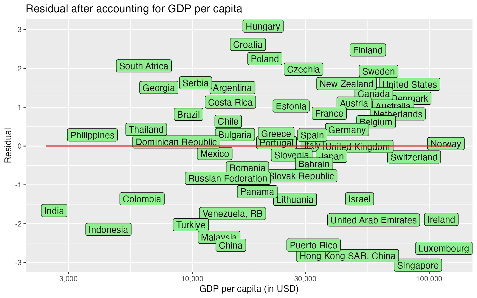
Here Hungary and Croatia show up as being relative pinball fanatics, considering their GDP per Capita. While Singapore and Luxembourg couldn’t care less for the silver ball. If you want to take a look yourself, here’s a CSV file with the full Public Pinball Machines per Capita dataset:
Code
pinball_country_stats |>
  select(country_name, country_code, population, n_locations, n_machines,  n_machines_per_million_capita, gdp_per_capita) |>
  write_csv("public_pinball_machines_per_capita_2024.csv")
public_pinball_machines_per_capita_2024.csv
Caveats: This indicator is mostly a joke, 100% depends on the completeness of Pinball Map, and countries without a single registered pinball machine are excluded.