Sometimes it feels a bit silly when a simple statistical model has a fancy-sounding name. But it also feels good to drop the following in casual conversation: “Ah, then I recommend a Plackett-Luce model, a straightforward generalization of the Bradley–Terry model, you know”, when a friend wonders how they could model their, say, pinball championship dataset. Incidentally, in this post we’re going to model the result of the IFPA 18 World Pinball Championship using a Plackett-Luce model, implemented in Stan as a generalization of the Bradley–Terry model, you know.
I know neither who Bradley, Terry, Plackett, nor Luce were, but I know when their models could be useful:
- A Bradley-Terry model can be used to model data where you have pairwise comparisons between different items, and you are interested in the underlying “fitness” of the items. A concrete example is sports where each match is a “pairwise comparison” between two players or teams, and you assume each player or team has an underlying skill or ability.
- A Plackett-Luce model can be useful when you have several rankings between items and you’re, again, interested in the “fitness” of each item. This model could be used to assess the quality of different products when each participant has ranked the items from best to worst. Or, in a sports setting, it can be used to model the underlying skills of each player when the outcome isn’t wins or losses, but rankings. Just like you have in pinball championships.
So, both models can model the skills of a number of players/teams, the only difference being that a Bradley-Terry works with wins/losses and a Plackett-Luce model works with rankings (1st/2nd/3rd/etc).
Now we’re going to grab some data with rankings from the IFPA 18 World Pinball Championship, implement a Bayesian Plackett-Luce model in Stan, and then take it for a spin.
IFPA 18 World Pinball Championship dataset
Despite the name, the IFPA 18 World Pinball Championship took place in 2023. The IFPA Championship is generally considered the most prestigious pinball competition, but the main reason why we’re going to analyze it here is because the results of all the 480 pinball matches that went down between the 80 competing players are available in a single spreadsheet! It’s not a very tidy dataset, however, and it will need some tidying up. I won’t bore you with the details, unless you really want to know:
How the sausage gets tidied up
library(readxl)
library(tidyverse)

# This data is NOT in a tidy format, and so the code to tidy it up
# will also be fairly messy...
# The result of IFPA 18 World Pinball Championship was downloaded
# from here: https://www.ifpapinball.com/ifpa18/
ifpa_xlsx_path <- "IFPA 18 World Pinball Championship live results.xlsx"

# Reading and tidying the sheet with the pinball machine names used in the tournament
machines_wide <- read_xlsx(ifpa_xlsx_path, sheet = "Machines", range = "B2:F22")
machines_long <- machines_wide |>
  select(old = OLD, mid = MID, new = NEW) |>
  pivot_longer(
    cols = everything(), names_to = "game_category", values_to = "game_name"
  ) |>
  # The two machines were missing from the original data
  add_row(game_category = "old", game_name = "Dodge City") |>
  add_row(game_category = "old", game_name = "8 Ball") |>
  arrange(game_name)

# Reading in the match data which is spread over multiple Session sheets,
# each containing several sub-tables with the results of the games.
ifpa_xlsx_info <-
  expand_grid(
    session = paste("Session", 1:8),
    tibble(
      group = 1:20,
      group_pos = seq(1, 96, 5)
    )
  ) |>
  rowwise() |>
  mutate(session_df = list(
    read_xlsx(
      ifpa_xlsx_path, sheet = session,
      range = paste0("A", group_pos, ":K", group_pos + 4),
      col_names = FALSE
    )
  )) |>
  ungroup()

# A function to pivot the sub-tables into a tidy data frame
pivot_session_df <- function(s) {
  player_names <- s$...1[2:5]
  game1 <- s$...3[2:5]
  score1 <- s$...5[2:5]
  game2 <- s$...6[2:5]
  score2 <- s$...8[2:5]
  game3 <- s$...9[2:5]
  score3 <- s$...11[2:5]

  tibble(
    player_name = rep(player_names, 3),
    round = rep(1:3, each = 4),
    game_name = c(game1, game2, game3),
    score = c(score1, score2, score3)
  )
}

# Stitching the data together, and turning it into long format.
# Also, adding unique numerical identifiers for everything
# as it's going to make things easier when writing the Stan model.
match_results <-
  ifpa_xlsx_info |>
  mutate(session_df = map(session_df, pivot_session_df)) |>
  unnest(session_df) |>
  left_join( machines_long, by = "game_name") |>
  mutate(
    session = str_remove(session, "Session "),
    player_id = as.integer(factor(player_name)),
    game_id = as.integer(factor(game_name)),
    game_category_id = recode(game_category, `old` = 1, `mid` = 2, `new` = 3),
    rank = recode(score, `7` = 1, `5` = 2, `3` = 3, `1` = 4),
  ) |>
  group_by(session, group, round) |>
  mutate(round_id = cur_group_id()) |>
  select(
    session, group, round, round_id, player_name, player_id, score, rank,
    game_name, game_id, game_category, game_category_id
  )

write_csv(match_results, "ifpa-18-world-pinball-championship-match-results.csv")
The final tidy IFPA 18 Pinball Championship dataset includes the results from each of the eight qualifying sessions before the final tournament:
library(tidyverse)
match_results <- read_csv("ifpa-18-world-pinball-championship-match-results.csv")
match_results
# A tibble: 1,920 × 12
   session group round round_id player_name    player_id score  rank game_name
     <dbl> <dbl> <dbl>    <dbl> <chr>              <dbl> <dbl> <dbl> <chr>
 1       1     1     1        1 Michael Trepp         57     1     4 Little Joe
 2       1     1     1        1 Bob Matthews          12     7     1 Little Joe
 3       1     1     1        1 Mark Pearson          54     3     3 Little Joe
 4       1     1     1        1 Escher Lefkoff        28     5     2 Little Joe
 5       1     1     2        2 Michael Trepp         57     5     2 Jokerz
 6       1     1     2        2 Bob Matthews          12     1     4 Jokerz
 7       1     1     2        2 Mark Pearson          54     7     1 Jokerz
 8       1     1     2        2 Escher Lefkoff        28     3     3 Jokerz
 9       1     1     3        3 Michael Trepp         57     3     3 Indianapol…
10       1     1     3        3 Bob Matthews          12     1     4 Indianapol…
# ℹ 1,910 more rows
# ℹ 3 more variables: game_id <dbl>, game_category <chr>,
#   game_category_id <dbl>
In each round during these sessions, four players compete on the same pinball machine. The player that comes 1st gets 7 points, the second one gets 5 points, and so on. For example, looking at the first couple of rows above, we can see that when competing on the Little Joe (1972) machine, Bob Matthews won and Michael Trepp ended up last. During the pre-tournament sessions, players rotate to face off against most other players and compete on many different pinball machines. At the end of the sessions, each player’s score is tallied up, and the top 32 players proceed to the final tournament (not included in this dataset).
We’re now ready to model this data using a Plackett-Luce model!
The Plackett-Luce model
Despite the somewhat involved names, both the Bradley–Terry model and the Plackett-Luce model are fairly straightforward. In the simplest case, without covariates, both models assume that each player (or team/item/product) has an underlying skill. In themselves, these skill parameters don’t have any meaning. They only become meaningful when used to come up with the probability of each player winning. Let’s say n players compete, each with their own skill parameter skill1, 2, …, n. Then the probability of each player winning is calculated as
$$p_1 = \frac{\exp({skill}_1)}{\sum(\exp({skill}_{1, 2, …, n}))}, \\[0.7em] p_2 = \frac{\exp({skill}_2)}{\sum(\exp({skill}_{1, 2, …, n}))}, \\[0.7em] … \\[0.5em] p_n = \frac{\exp({skill}_n)}{\sum(\exp({skill}_{1, 2, …, n}))}$$
The exp () makes sure that the result is always positive, even for
negative skills, and by dividing by
∑(exp(skill1, 2, …, n)) we make the transformed
skills sum to one like good probabilities should (this transformation is
known as
the softmax
function).
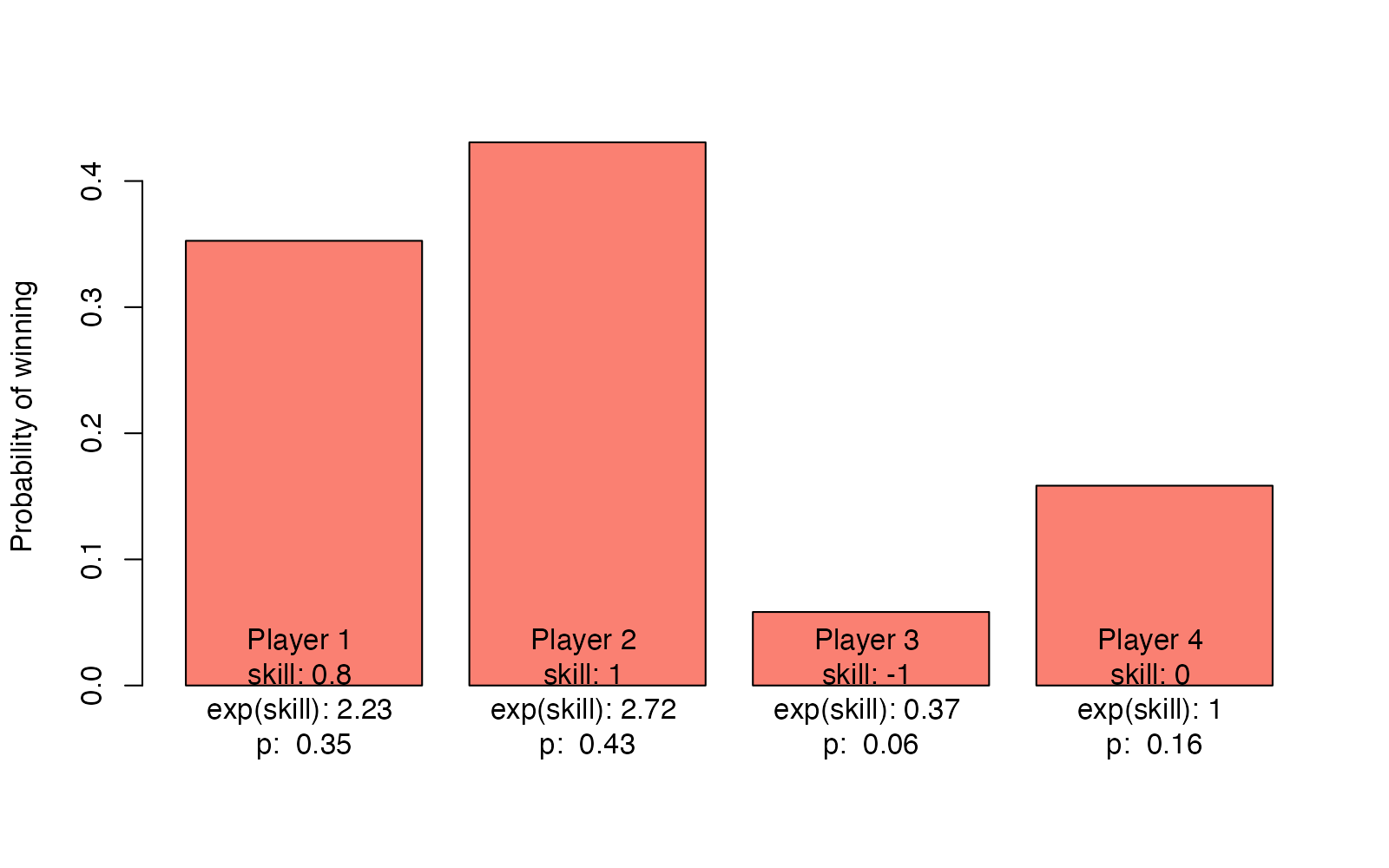
For example, if we have four players with skills
c(0.8, 1.0, -1.0, 0.0) the probability distribution p over each
player winning would be:
skills <- c(0.8, 1.0, -1.0, 0.0)
p <- exp(skills) / sum(exp(skills))

barplot(p, col = "salmon", ylab = "Probability of winning", names.arg =
  paste(
    "Player", 1:4, "\nskill:", skills, "\nexp(skill):", round(exp(skills), 2),
    "\np: ", round(p, 2)
  )
)
The sole difference between the Bradley–Terry model and the Plackett-Luce model is in what data they model: Bradley-Terry models the winner of a competition between two players, while Plackett-Luce models the rankings in a competition with several players. It does this by assuming that the performance of each player isn’t influenced by the other players, which allows for modeling rankings as a series of competitions. Perhaps it’s easiest to explain by showing the “generative model” in R, for a competition with our four players from above:
players <- 1:4 # Our four competing players

# Sampling the winner of the bunch
p <- exp(skills[players]) / sum(exp(skills[players]))
first <- sample(players, prob = p, size = 1)

# Excluding the player who came first, who will win second place?
players <- players[players != first]
p <- exp(skills[players]) / sum(exp(skills[players]))
second <- sample(players, prob = p, size = 1)

# Excluding the players who came first and second, who will win third place?
players <- players[players != second]
p <- exp(skills[players]) / sum(exp(skills[players]))
third <- sample(players, prob = p, size = 1)

# The player who's left gets fourth place
fourth <- players[players != third]

ranking <- c(first, second, third, fourth)
ranking
[1] 4 1 2 3
That’s basically the simple version of the Plackett-Luce model. In our case we, of course, know the rankings of all the competitions in the IFPA 18 Pinball Championship so we don’t want to simulate the data using fixed skill parameters. Instead, we’re now ready to do the Bayesian trick where we assume the player skills are unknown parameters and use the data to figure them out.
A Plackett-Luce model in Stan
While we could work with the tidied match_results in Stan, the model
becomes easier to implement if we extract only the parts of the data
that we need. Here, that’s the number of players (n_players), the
number of rounds (n_round), and a matrix with the 1st, 2nd, 3rd, and
4th player_id for each round (player_ranks).
stan_data <- list(
  n_players = max(match_results$player_id),
  n_rounds = max(match_results$round_id),
  player_ranks = match_results |>
    select(round_id, rank, player_id) |>
    pivot_wider(names_from = rank, values_from = player_id) |>
    arrange(round_id) |>
    select(`1`, `2`, `3`, `4`) |>
    as.matrix()
)
head(stan_data$player_ranks)
      1  2  3  4
[1,] 12 28 54 57
[2,] 54 57 28 12
[3,] 28 54 57 12
[4,] 64 37  2 62
[5,] 64 62 37  2
[6,] 62  2 37 64
For example, looking at the first couple of rows in
stan_data$player_ranks above, we can (again) see that in round one, on
the first row, player_id: 12 (that is, Bob Matthews) won and
player_id: 57 (Michael Trepp) came last.
Also, while we could implement the likelihood part of this model
directly using sum()s and exp()s, a shortcut is to use the
categorical_logit() distribution. The parameter to this distribution
is a vector which will be
softmax
transformed (just what we want in the Plackett-Luce model) into the
probability that each of the categories represented by this vector will
be selected. For example, this sampling statement defines the likelihood
that the first player, with skill 0.8 would win:
1 ~ categorical_logit([0.8, 1.0, -1.0, 0.0]).
Given that we’ve got our data nicely packaged up in stan_data and that
we can use the categorical_logit() distribution, the Stan model
definition becomes fairly straightforward:
plackett_luce_model_code <- "
data {
  int n_players;
  int n_rounds;
  int player_ranks[n_rounds, 4];
}

parameters {
  vector[n_players] skills;
  real<lower=0> skills_sigma;
}

model {
  // A vector to hold the skills for each round
  // Just to limit the amunt of indexing we'll need to do
  vector[4] round_skills;

  // It's important that the distribution over skills is anchored at a
  // fixed value, here 0.0. Otherwise, as skills are relative to each other,
  // they wouldn't be identifiable.
  skills ~ normal(0, skills_sigma);
  skills_sigma ~ cauchy(0, 1);

  for (round_i in 1:n_rounds) {
    round_skills = skills[player_ranks[round_i]];

    // The likelihood of the winner winning out of the 4 players
    1 ~ categorical_logit(round_skills[1:4]);
    // The likelihood of the 2nd place winning out of the 3 remaining players
    1 ~ categorical_logit(round_skills[2:4]);
    // The likelihood of the 3rd place winning out of the 2 remaining players
    1 ~ categorical_logit(round_skills[3:4]);
    // And the remaining 4th place is guaranteed to 'win' against themselves...
  }
}
"
In the above model, I’ve placed a hierarchical distribution on the
skills parameters. This works well for this dataset, where there are a
lot of players and plenty of data. With less data, one might want to
just put a fixed prior here (say, skills ~ normal(0, 1.0)). The model
above is somewhat inflexible in that it only works for the case where
there are exactly four players in each round, but I hope you can see
that it’s straightforward to tweak it to allow for other number of
players, as well.
Now we can finally go ahead and fit this model!
library(rstan)

model_fit <- stan(
  model_code = plackett_luce_model_code, data = stan_data,
  chains = 4, iter = 20000, cores = 4
)
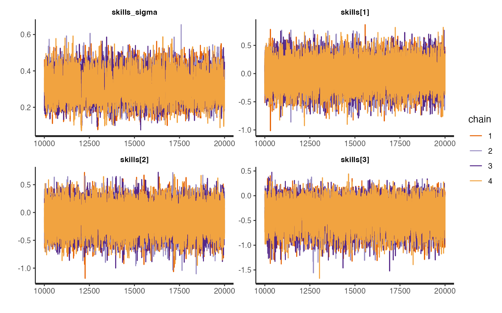
Skimping a bit on checking model convergence, we can, at least, see that both the trace plots and the number of effective samples look reasonable.
traceplot(model_fit, pars = c("skills_sigma", "skills[1]", "skills[2]", "skills[3]"))
model_fit |>
  extract(pars = c("skills_sigma", "skills[1]", "skills[2]", "skills[3]"), permuted = FALSE) |>
  monitor()
Inference for the input samples (4 chains: each with iter = 10000; warmup = 5000):

               Q5  Q50 Q95 Mean  SD  Rhat Bulk_ESS Tail_ESS
skills_sigma  0.2  0.3 0.4  0.3 0.1     1     2252     2456
skills[1]    -0.4  0.0 0.3  0.0 0.2     1    37109    14113
skills[2]    -0.5 -0.1 0.2 -0.1 0.2     1    29867    13139
skills[3]    -0.8 -0.4 0.0 -0.4 0.2     1     8267    13065

For each parameter, Bulk_ESS and Tail_ESS are crude measures of
effective sample size for bulk and tail quantities respectively (an ESS > 100
per chain is considered good), and Rhat is the potential scale reduction
factor on rank normalized split chains (at convergence, Rhat <= 1.05).
That was a simple Plackett-Luce model in Stan. But finally, let’s have a look at the fitted Plackett-Luce model of the IFPA 18 World Pinball Championship.
The fitted IFPA 18 World Pinball Championship model
First, let’s extract the player skill parameters. For simplicity I’ll use the median point estimates and 95% probability intervals here, rather than working with the full distributions.
skills_summary <- summary(model_fit, pars = "skills")$summary

player_skill <- match_results |>
  summarise(score = sum(score), .by = c(player_id, player_name)) |>
  arrange(player_id) |>
  mutate(
    median_skill = skills_summary[, "50%"],
    lower_skill = skills_summary[, "2.5%"],
    upper_skill = skills_summary[, "97.5%"]
  ) |>
  arrange(desc(median_skill))
player_skill
# A tibble: 80 × 6
   player_id player_name              score median_skill lower_skill upper_skill
       <dbl> <chr>                    <dbl>        <dbl>       <dbl>       <dbl>
 1        39 Johannes Ostermeier        138        0.669      0.134        1.28
 2        28 Escher Lefkoff             130        0.570      0.0811       1.15
 3        54 Mark Pearson               114        0.362     -0.0724       0.864
 4        47 Keith Elwin                116        0.338     -0.0973       0.851
 5        21 Daniele Celestino Accia…   114        0.327     -0.111        0.835
 6        78 Viggo Löwgren              118        0.307     -0.119        0.804
 7        80 Zach Sharpe                116        0.294     -0.137        0.786
 8        36 Jason Zahler               106        0.240     -0.183        0.722
 9        48 Keri Wing                  108        0.230     -0.184        0.692
10        45 Josh Sharpe                110        0.226     -0.191        0.701
# ℹ 70 more rows
Not surprisingly, we find that Johannes Ostermeier, who ended up winning the whole tournament, also got the highest skill estimate. We can now also plot all the skill estimates:
Plot code
player_skill |>
  mutate(player_name = fct_reorder(player_name, median_skill)) |>
  ggplot(aes(x = median_skill, y = player_name)) +
  geom_point() +
  geom_errorbarh(aes(xmin = lower_skill, xmax = upper_skill), height = 0) +
  labs(
    title = "Player skill estimates for IFPA 18 World Pinball Championship",
    subtitle = "Posterior medians with 95% probablilty intervals",
    x = "Skill", y = ""
  ) +
  theme_minimal() +
  theme(axis.text.y = element_text(size = 6))
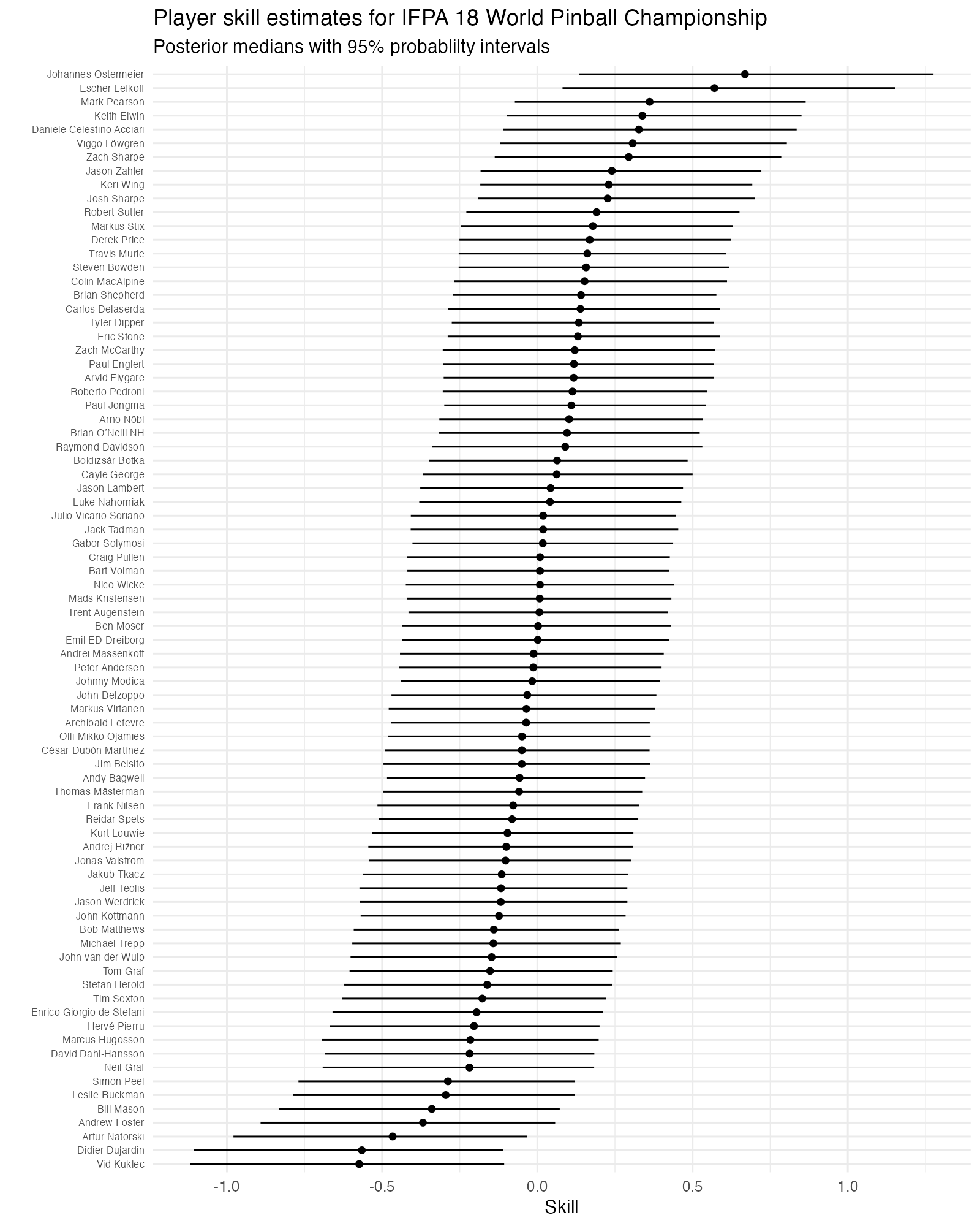
It’s somewhat hard to interpret these skill estimates on their own, but two things to note here:
- Despite the large number of rounds played (480), the uncertainty in the skill parameters is large.
- Overall, players have very similar skill. This is not so surprising, as these are all top pinball players. If I had competed here, my skill estimate would be far far to the left.
To verify that these skill parameters make some sense, we could also plot them against each player’s final score from the qualifying sessions:
Plot code
player_skill |>
  ggplot(aes(x = median_skill, y = score)) +
  geom_point() +
  labs(
    title = "Player skill vs final score for IFPA 18 World Pinball Championship",
    x = "Median player skill", y = "Final Score"
  ) +
  theme_minimal()
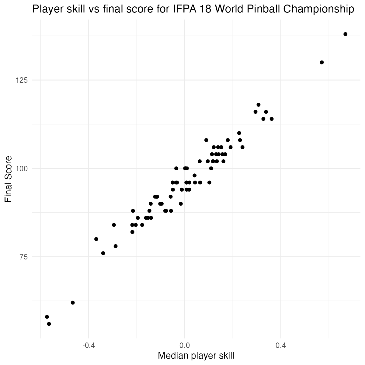
The final score and the estimated skill are so strongly correlated that one might wonder if there was any point at all in going through the trouble of fitting a Plackett-Luce model. However, we can do much more interesting stuff with the skill estimates than we can with just the scores. For example, we can calculate the probability of players winning in different matchups. Say the top player played against the three players with the lowest skill:
highest_and_lowest_players <- union(
 slice_max(player_skill, median_skill, n = 1),
 slice_min(player_skill, median_skill, n = 3)
)
highest_and_lowest_players
# A tibble: 4 × 6
  player_id player_name         score median_skill lower_skill upper_skill
      <dbl> <chr>               <dbl>        <dbl>       <dbl>       <dbl>
1        39 Johannes Ostermeier   138        0.669       0.134      1.28
2        77 Vid Kuklec             58       -0.574      -1.12      -0.107
3        24 Didier Dujardin        56       -0.565      -1.11      -0.109
4         7 Artur Natorski         62       -0.466      -0.979     -0.0334
skills <- highest_and_lowest_players$median_skill
p <- exp(skills) / sum(exp(skills))

barplot(p, col = "aquamarine", ylab = "Probability of winning", names.arg =
  paste(highest_and_lowest_players$player_name, "\np: ", round(p, 2))
)
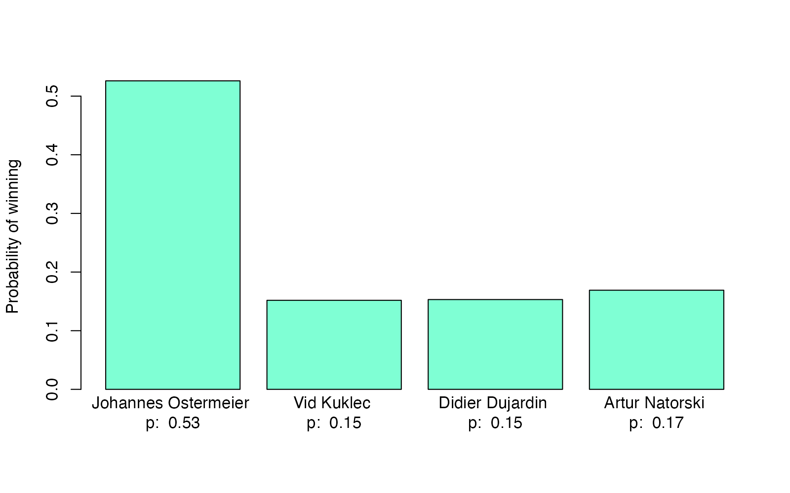
Here, according to this model, Johannes would have a 53% probability of winning when facing Vid, Didier, and Artur. Again, this shows that in a single game of pinball, even when the top player meets the lowest scoring players in the World Pinball Championship, it’s still far from guaranteed that the top player would win. But at the IFPA 18 World Pinball Championship Johannes did go all the way and won the final game as shown in this live stream.
All code for this post can be found in this Quarto markdown file.
Update: Bob Carpenter has published a case study analyzing sushi rating data with an alternative (and faster) Plackett-Luce model in Stan.