Correlation does not imply causation, right but, as Edward Tufte writes, “it sure is a hint.” The Pearson product-moment correlation coefficient is perhaps one of the most common ways of looking for such hints and this post describes the Bayesian First Aid alternative to the classical Pearson correlation test. Except for being based on Bayesian estimation (a good thing in my book) this alternative is more robust to outliers and comes with a pretty nice default plot. :)
Bayesian First Aid is an attempt at implementing reasonable Bayesian alternatives to the classical hypothesis tests in R. For the rationale behind Bayesian First Aid see the original announcement. The development of Bayesian First Aid can be followed on GitHub. Bayesian First Aid is a work in progress and I’m grateful for any suggestion on how to improve it!
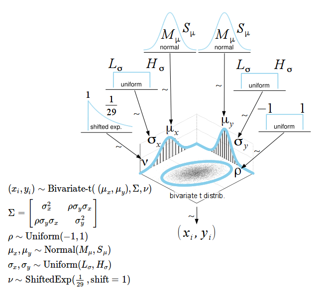
The Model
The classical test of Pearson product-moment correlation coefficient between two paired variables $x_i$ and $y_i$ assumes bivariate normality. It assumes that the relation is linear and that both $x_i$ and $y_i$ are normally distributed. I’ve already written about a Bayesian alternative to the correlation test here and about how that model can be made more robust here. The Bayesian First Aid alternative is basically the robustified version with slightly different priors.
Instead of a bivariate normal distribution we’ll assume a bivariate t distribution. This is the same trick as in the Bayesian First Aid alternative to the t-test, compared to the normal distribution the wider tails of the t will downweight the influence of stray data points. The model has six parameters: the means of the two marginal distributions ($\mu_x,\mu_y$), the SDs ($\sigma_x,\sigma_y$), the degree-of-freedoms parameter that influences the heaviness of the tails ($\nu$), and finally the correlation ($\rho$). The SDs and $\rho$ are then used to define the covariance matrix of the t distribution as:
$$ \Sigma = \begin{bmatrix} \sigma_x^2 & \rho\sigma_y\sigma_x \\ \rho\sigma_y\sigma_x & \sigma_y^2 \end{bmatrix} $$
The priors on $\mu_x,\mu_y, \sigma_x,\sigma_y$ and $\nu$ are also the same as in the alternative to the two sample t-test, that is, by peeking at the data we set the hyperparameters $M_\mu, S_\mu, L_\sigma$ and $H_\sigma$ resulting in a, for all practical purposes, flat prior. When modeling correlations it is common to directly put a prior distribution on the covariance matrix (the Inverse-Wishart distribution for example). Here we instead do as described by Barnard, McCulloch & Meng (2000) and put separate priors on $\sigma_x,\sigma_y$ and $\rho$, where $\rho$ is given a uniform prior. The advantage with separate priors is that it gives you greater flexibility and makes it easy to add prior information into the mix.
So, here is the final model for the Bayesian First Aid alternative to the correlation test:
The bayes.cor.test Function
The bayes.cor.test function can be called exactly as the cor.test function in R. If you just ran cor.test(x, y), prepending bayes. (like bayes.cor.test(x, y)) runs the Bayesian First Aid alternative and prints out a summary of the model result. By saving the output, for example, like fit <- bayes.cor.test(x, y) you can inspect it further using plot(fit), summary(fit) and diagnostics(fit).
To showcase bayes.cor.test I will use data from the article
2D:4D ratios predict hand grip strength (but not hand grip endurance) in men (but not in women) by Hone & McCullough (2012). The ratio here referred to is that between one’s index finger (2D) and ring finger (4D) which is nicely visualized in the Wikipedia entry for
digit ratio:
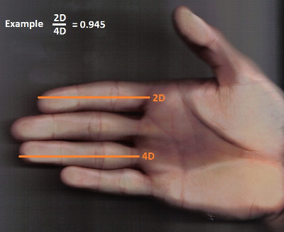
So why is the 2D:4D ratio an interesting measure? It is believed that the 2D:4D ratio is affected by the prenatal exposure to androgens (hormones that control the development of male characteristics) with a lower 2D:4D ratio being indicative of higher androgen exposure. Stated in a sloppy way, the working hypothesis is that the 2D:4D ratio is a proxy variable for prenatal androgen exposure and could therefore be related to a host of other traits related to “manliness” such as aggression, prostate cancer risk, sperm count, etc. (see Wikipedia for a longer list). Hone & McCullough was interested in the relation between the 2D:4D ratio and a typical “manly” attribute, muscle strength. They therefore measured the grip strength (in kg) and the 2D:4D ratio in 222 psychology students (100 male, 122 female) and found that:
2D:4D ratios significantly predicted [grip strength] in men, but not in women. […] We conclude furthermore that the association of prenatal exposure to testosterone (as indexed by 2D:4D ratios) and strength pertains only to men, and not to women."
Two points regarding their analysis, before moving on:
- They support the conclusion above by comparing the regression p-values between the male group (p < 0.001) and the female group (p = 0.09) and notice that while the regression coefficient is less than 0.05 for the male group it is more than 0.05 for female group. It is not clear to me how p = 0.09 is strong evidence that prenatal exposure to testosterone does not influence strength in women at all.
- Hone & McCullough tests the null hypothesis that there is no correlation whatsoever between 2D:4D ratio and strength. This question could be answered without any data, of course there is some correlation between 2D:4D ratio and strength (no matter how tiny). In complex systems, such as humans, it would be extremely unlikely that any given trait (such as hair color, shoe size, movie taste, running speed, no of tweets, etc.) does not correlate at all with any other trait. More interesting is to what degree 2D:4D ratio and strength correlates (which Hone & McCullough also estimated but did not base the final conclusion on).
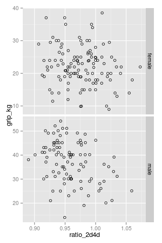
We’ll leave Hone & McCullough’s analysis behind us (their analysis included many more variables, for one thing) and will just look at the strength and digit ratio data. The data was scraped from two scatter plots using the great and free online tool WebPlotDigitizer (so it might differ slightly from the original data, though I was pretty thorough) and can be downloaded here: 2d4d_hone_2012.csv. Here is how it looks:
d <- read.csv("2d4d_hone_2012.csv")
qplot(ratio_2d4d, grip_kg, data = d, shape = I(1)) + facet_grid(sex ~ ., scales = "free")
Let’s first estimate the correlation for the male group using the classical cor.test:
cor.test( ~ ratio_2d4d + grip_kg, data = d[d$sex == "male", ])
##
## 	Pearson's product-moment correlation
##
## data:  ratio_2d4d and grip_kg
## t = -3.612, df = 95, p-value = 0.0004879
## alternative hypothesis: true correlation is not equal to 0
## 95 percent confidence interval:
##  -0.5115 -0.1591
## sample estimates:
##     cor
## -0.3475
And now using the Bayesian First Aid version:
fit_male <- bayes.cor.test( ~ ratio_2d4d + grip_kg, data = d[ d$sex == "male",])
fit_male
##
## 	Bayesian First Aid Pearson's Correlation Coefficient Test
##
## data: ratio_2d4d and grip_kg (n = 97)
## Estimated correlation:
##   -0.34
## 95% credible interval:
##   -0.52 -0.15
## The correlation is more than 0 by a probability of 0.001
## and less than 0 by a probability of 0.999
Both estimates are very similar and both indicate a slight negative correlation. Let’s look at the Bayesian First Aid plot:
plot(fit_male)
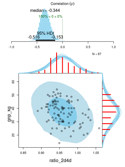
This plot shows lots of useful stuff! At the top we have the posterior distribution for the correlation $\rho$ with a 95% highest density interval. At the bottom we see the original data with superimposed posterior predictive distributions (that is, the distribution we would expect a new data point to have). This is useful when assessing how well the model fits the data. The two ellipses show the 50% (darker blue) and 95% (lighter blue) highest density regions. The red histograms show the marginal distributions of the data with a smatter of marginal densities drawn from the posterior. Looking at this plot we see that the model fits quite well, however, we could be concerned with the right skewness of the ratio_2d4d marginal which is not captured by the model.
Now let’s look at the corresponding plot for the female data:
fit_female <- bayes.cor.test( ~ ratio_2d4d + grip_kg, data = d[ d$sex == "female",])
plot(fit_female)
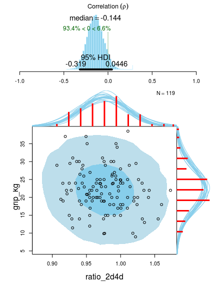
Indeed, 2D:4D ratio and strength seems to be slightly less correlated than for the male group, but to claim there is evidence for no correlation seems a bit unfounded. We could, however, take a look at the posterior difference in correlation between the male and the female group. To do this we first extract the MCMC samples from the Bayesian First Aid fit object using the as.data.frame function.
female_mcmc <- as.data.frame(fit_female)
male_mcmc <- as.data.frame(fit_male)
head(female_mcmc)
##         rho    mu1   mu2  sigma1 sigma2     nu
## 1  0.024912 0.9758 22.84 0.03196  6.209  33.14
## 2 -0.002173 0.9718 22.24 0.03336  6.082  57.15
## 3  0.013787 0.9773 21.39 0.03577  5.712  66.23
## 4  0.017139 0.9751 22.10 0.03779  5.687 129.93
## 5  0.014113 0.9779 21.75 0.03482  6.245 149.52
## 6  0.025849 0.9766 21.13 0.03525  6.320 114.16
We’ll then plot the difference in $\rho$ and calculate the probability that $\rho$ is more negative for men:
hist(male_mcmc$rho - female_mcmc$rho, 30, xlim = c(-1, 1), main = "", yaxt = "n")

mean(male_mcmc$rho - female_mcmc$rho < 0)
## [1] 0.9321
Even though we can’t claim that 2D:4D ratio and strength is not correlated in women at all, there is some evidence that 2D:4D ratio and strength is more negatively correlated in men than in women. Given that I have a relatively high (less “manly”) 2D:4D ratio of 1.0 does it mean I have an excuse for my subpar arm strength? Nope, I should just go to the gym more often…
bayes.cor.test Model Code
A great thing with Bayesian data analysis is that it is simple to step away from the well trodden model and explore alternatives. The Bayesian First Aid function that makes this easy is model.code, if you just ran fit <- bayes.cor.test(exposure_to_puppies, rated_happiness) a call to model.code(fit) prints out corresponding R and JAGS code that can be directly copy-n-pasted into an R script and modified from there.
model.code(fit)
## Model code for the Bayesian First Aid alternative to Pearson's correlation test. ##
require(rjags)

# Setting up the data
x <- exposure_to_puppies
y <- rated_happieness
xy <- cbind(x, y)

# The model string written in the JAGS language
model_string <- "model {
  for(i in 1:n) {
    xy[i,1:2] ~ dmt(mu[], prec[ , ], nu)
  }

  # JAGS parameterizes the multivariate t using precision (inverse of variance)
  # rather than variance, therefore here inverting the covariance matrix.
  prec[1:2,1:2] <- inverse(cov[,])

  # Constructing the covariance matrix
  cov[1,1] <- sigma[1] * sigma[1]
  cov[1,2] <- sigma[1] * sigma[2] * rho
  cov[2,1] <- sigma[1] * sigma[2] * rho
  cov[2,2] <- sigma[2] * sigma[2]

  ## Priors
  rho ~ dunif(-1, 1)
  sigma[1] ~ dunif(sigmaLow, sigmaHigh)
  sigma[2] ~ dunif(sigmaLow, sigmaHigh)
  mu[1] ~ dnorm(mean_mu, precision_mu)
  mu[2] ~ dnorm(mean_mu, precision_mu)
  nu <- nuMinusOne+1
  nuMinusOne ~ dexp(1/29)
}"

# Initializing the data list and setting parameters for the priors
# that in practice will result in flat priors on mu and sigma.
data_list = list(
  xy = cbind(x, y),
  n = length(x),
  mean_mu = mean(c(x, y), trim=0.2) ,
  precision_mu = 1 / (max(mad(x), mad(y))^2 * 1000000),
  sigmaLow = max(mad(x), mad(y)) / 1000 ,
  sigmaHigh = min(mad(x), mad(y)) * 1000)

# Initializing parameters to sensible starting values helps the convergence
# of the MCMC sampling. Here using robust estimates of the mean (trimmed)
# and standard deviation (MAD).
inits_list = list(mu=c(mean(x, trim=0.2), mean(y, trim=0.2)), rho=cor(x, y, method="spearman"),
                  sigma = c(mad(x), mad(y)), nuMinusOne = 5)

# The parameters to monitor.
params <- c("rho", "mu", "sigma", "nu")

# Running the model
model <- jags.model(textConnection(model_string), data = data_list,
                    inits = inits_list, n.chains = 3, n.adapt=1000)
update(model, 500) # Burning some samples to the MCMC gods....
samples <- coda.samples(model, params, n.iter=5000)

# Inspecting the posterior
plot(samples)
summary(samples)
One thing that we might want to change is the prior on rho which is currently $\text{Uniform}(-1,1)$. As described by
Barnard, McCulloch & Meng (2000), the
beta distribution stretched to the interval [-1,1] is a flexible alternative that facilitates the construction of a more informative prior. To use this prior we’ll have to replace
rho ~ dunif(-1, 1)
by
rho_half_with ~ dbeta(1, 1)
# shifting and streching rho_half_with from [0,1] to [-1,1]
rho ~ 2 * rho_half_with - 1
and replace the initialization of rho with the initialization of rho_half_width:
inits_list = list(mu = c(mean(x, trim=0.2), mean(y, trim=0.2)),
                  rho_half_width = (cor(x, y, method="spearman") + 1) / 2,
                  sigma = c(mad(x), mad(y)), nuMinusOne = 5)
Now, by changing the parameters of dbeta we can specify a range of different priors:

Here the top left prior is the uniform, representing little prior information on the correlation between measures of puppy exposure and happiness. The top right prior is skeptical of there being a large correlation but is agnostic with respect to the direction. The lower left prior is just slightly in favor of a positive correlation, with the lower right being quite optimistic putting more than 99% of the prior probability over rho > 0.