The Stan project for statistical computation has a great collection of curated case studies which anybody can contribute to, maybe even me, I was thinking. But I don’t have time to worry about that right now because I’m on vacation, being on the yearly visit to my old family home in the north of Sweden.
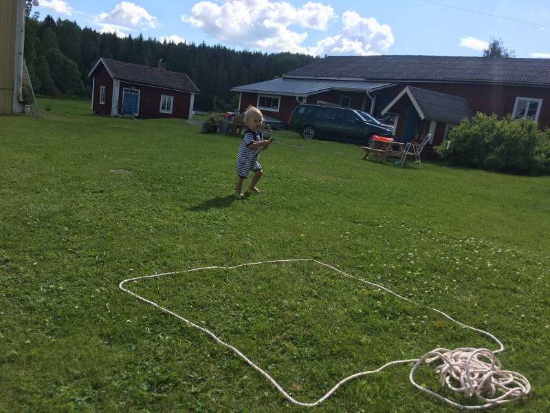
What I do worry about is that my son will be stung by a bumblebee. His name is Torsten, he’s almost two years old, and he loves running around barefoot on the big lawn. Which has its fair share of bumblebees. Maybe I should put shoes on him so he wont step on one, but what are the chances, really.
Well, what are the chances? I guess if I only had
- Data on the bumblebee density of the lawn.
- Data on the size of Torsten’s feet and how many steps he takes when running around.
- A reasonable Bayesian model, maybe implemented in Stan.
I could figure that out. “How hard can it be?”, I thought. And so I made an attempt.
Getting the data
To get some data on bumblebee density I marked out a 1 m² square on a representative part of the lawn. During the course of the day, now and then, I counted up how many bumblebees sat in the square.
Most of the time I saw zero bumblebees, but 1 m² is not that large of an area. Let’s put the data into R:
bumblebees <- c(1, 0,  0, 0, 0, 0, 0, 0, 0, 0, 0, 0, 0, 0, 0, 0, 0, 0, 0, 0, 0,
                1, 0, 0, 0, 0, 0, 0, 1, 0, 0, 0, 0, 0, 0, 0, 0, 0, 0, 0, 0, 1,
                0, 0, 1, 0, 0, 0, 0, 0, 0)
During the same day I kept an eye on Torsten, and sometimes when he was engaged in active play I started a 60 s. timer and counted how many steps he took while running around. Here are the counts:
toddler_steps <- c(26, 16, 37, 101, 12, 122, 90, 55, 56, 39, 55, 15, 45, 8)
Finally I needed to know the area of Torsten’s feet. At a moment when he was not running around I put his foot on a piece of graph paper and traced its edge, which made him giggle. I then calculated how many of the 0.5 cm² squares were fully covered and how many were partially covered.
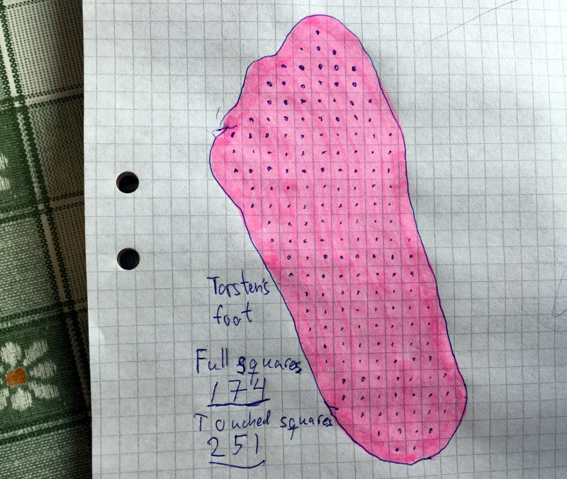
To estimate of the area of his foot I took the average of the number of full squares and the number partial squares, and then converted to m²:
full_squares <- 174
partial_squares <- 251
squares <- (full_squares + partial_squares) / 2
foot_cm2 <- squares / 4
foot_m2 <- foot_cm2 / 100^2
foot_m2
## [1] 0.0053125
Turns out my son’s feet are about 0.0053 m² each.
Specifying the model
The idea I had here was that if you know the average number of steps Torsten takes per minute while playing, and if you know the average number of bumblebees per m², then you could calculate the average area covered by Torsten’s tiny feet while running around, and then finally you could calculate the probability of a bumblebee being in that area. This would give you a probability for how likely Torsten is to be stung by a Bumblebee. However, while we have data on all of the above, we don’t know any of the above for certain.
So, to capture some of this uncertainty I thought I would whip together a small Bayesian model and, even though it’s a bit overkill in this case, why not fit it using Stan? (If you are unfamiliar with Bayesian data analysis and Stan I’ve made a short video tutorial you can find here.)
Let’s start our Stan program by declaring what data we have:
data {
  int n_bumblebee_observations;
  int bumblebees[n_bumblebee_observations];
  int n_toddler_steps_observations;
  int toddler_steps[n_toddler_steps_observations];
  real foot_m2;
}
Now we need to decide on a model for the number of bumblebees in a m² and a model for the number of toddler_steps in 60 s. For the bees I’m going with a simple Poisson model, that is, the model assumes there is an average number of bees per m² ($\mu_\text{bees}$) and that this is all there is to know about bees.
For the number of steps I’m going to step it up a notch with a negative binomial model. The negative binomial distribution can be viewed in a number of ways, but one particularly useful way is as an extension of the Poisson distribution where the mean number of steps for each outcome is not fixed, but instead is varying, where this is controlled by the precision parameter $\phi_\text{steps}$. The larger $\phi_\text{steps}$ is the less the mean number of steps for each outcome is going to vary around the overall mean $\mu_\text{steps}$. That is, when $\phi_\text{steps} \rightarrow \infty$ then the negative binomial becomes a Poisson distribution. The point with using the negative binomial is to capture that Torsten’s activity level when playing on the lawn is definitely not constant. Sometimes he can run full speed for minutes, but sometimes he spends a long time being fascinated by the same little piece of rubbish and then he’s not taking many steps.
So we almost have a Bayesian model for our data, we just need to put priors on the parameters $\mu_\text{bees}$, $\mu_\text{steps}$, and $\phi_\text{steps}$. All three parameters are positive and a quick n’ dirty prior when you have positive parameters is a half-Cauchy distribution centered at zero: It’s just like half a normal distribution centered at zero, but with a much fatter tail. It has one free parameter, the scale, which also happens to be the median of the half-Cauchy. Set the scale/median to a good guess for the parameter in question and you are ready to go! If your guess is good then this prior will give the parameter the slightest nudge in the right direction, if your guess is bad then, as long as you have enough data, the fat tail of the half-Cauchy distribution will help you save face.
My guess for $\mu_\text{bees}$ is (4.0 + 4.0) / (10 × 10) = 0.08. I base this on that while crossing the lawn I usually scan an area of about 10×10 m², I then usually see around four bees, and I assume I’m missing half of the bees. So eight bees on a 100 m² lawn gives 0.08 bees per m². My guess for the number of steps per minute is going to be 60. For the precision parameter $\phi_\text{steps}$ I have no clue, but it shouldn’t be too large nor to small, so my guess is going to be 1.0. Here are the priors:
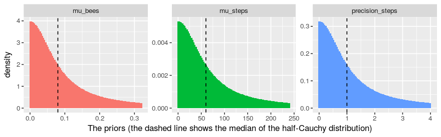
With the priors specified we now have all the required parts and here is the resulting Bayesian model:
$$ \begin{align*} & \text{bees} \sim \text{Poisson}(\mu_\text{bees}) \\ & \text{steps} \sim \text{Neg-Binomial}(\mu_\text{steps}, \phi_\text{steps}) \\ & \mu_\text{bees} \sim \text{Half-Cauchy}((4 + 4) / (10 \times 10)) \\ & \mu_\text{steps} \sim \text{Half-Cauchy}(60) \\ & \phi_\text{steps} \sim \text{Half-Cauchy}(1) \end{align*}$$
And here is the Stan code implementing the model above:
parameters {
  real<lower=0> mu_bees;
  real<lower=0> mu_steps;
  real<lower=0> precision_steps;
}

model {
  # Since we have contrained the parameters to be positive we get implicit
  # half-cauchy distributions even if we declare them to be 'full'-cauchy.
  mu_bees ~ cauchy(0, (4.0 + 4.0) / (10.0 * 10.0) );
  mu_steps ~ cauchy(0, 60);
  precision_steps ~ cauchy(0, 1);
  bumblebees ~ poisson(mu_bees);
  toddler_steps ~ neg_binomial_2(mu_steps, precision_steps);
}
The final step is to predict how many bumblebees Torsten will step on during, say, one hour of active play. We do this in the generated quantities code block in Stan. The code below will step through 60 minutes (a.k.a. one hour) and for each minute: (1) Sample pred_steps from the negative binomial, (2) calculate the area (m²) covered by these steps, and (3) sample the number of bees in this area from the Poisson giving a predicted stings_by_minute. Finally we sum these 60 minutes worth of strings into stings_by_hour.
generated quantities {
  int stings_by_minute[60];
  int stings_by_hour;
  int pred_steps;
  real stepped_area;

  for(minute in 1:60) {
    pred_steps =  neg_binomial_2_rng(mu_steps, precision_steps);
    stepped_area = pred_steps * foot_m2;
    stings_by_minute[minute] = poisson_rng(mu_bees * stepped_area);
  }
  stings_by_hour = sum(stings_by_minute);
}
Looking at the result
We have data, we have a model, and now all we need to do is fit it. After we’ve put the whole Stan model into bee_model_code as a string we do it like this using the rstan interface:
# First we put all the data into a list
data_list <- list(
  n_bumblebee_observations = length(bumblebees),
  bumblebees = bumblebees,
  n_toddler_steps_observations = length(toddler_steps),
  toddler_steps = toddler_steps,
  foot_m2 = foot_m2
)
# Then we fit the model which description is in bee_model_code .
library(rstan)
fit <- stan(model_code = bee_model_code, data = data_list)
With the model fitted, let’s take a look at the posterior probability distribution of our parameters.
stan_hist(fit, c("mu_bees", "mu_steps", "precision_steps"))
print(fit, c("mu_bees", "mu_steps", "precision_steps"))
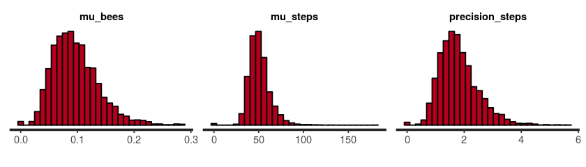
##                  mean se_mean    sd  2.5%   25%   50%   75% 97.5% n_eff Rhat
## mu_bees          0.12    0.00  0.05  0.04  0.08  0.11  0.15  0.23  3551    1
## mu_steps        50.88    0.22 11.65 32.56 43.09 49.34 57.13 78.00  2801    1
## precision_steps  1.80    0.01  0.68  0.78  1.32  1.70  2.17  3.41  2706    1
This seems reasonable, but note that the distributions are pretty wide, which means there is a lot of uncertainty! For example, looking at mu_bees it’s credible that there is everything from 0.04 bees/m² to 0.2 bees/m².
Anyway, let’s take a look at what we are really interested in, the predictive distribution over how many stings per hour Torsten will suffer during active play:
# Getting the sample representing the prob. distribution over stings/hour .
stings_by_hour <- as.data.frame(fit)$stings_by_hour
# Now actually calculating the prob of 0 stings, 1 stings, 2 stiongs, etc.
strings_probability <- prop.table( table(stings_by_hour) )
# Plotin' n' printin'
barplot(strings_probability, col = "yellow",
        main = "Posterior predictive stings per hour",
        xlab = "Number of stings", ylab = "Probability")
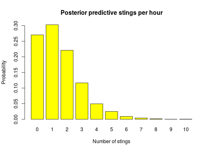
round(strings_probability, 2)
## stings_by_hour
##    0    1    2    3    4    5    6    7    8    9   10
## 0.27 0.30 0.22 0.12 0.05 0.02 0.01 0.00 0.00 0.00 0.00
Ok, it seems like it is most probable that Torsten will receive one sting per hour, but we should not be surprised if it’s two or even three stings. I’d better put some shoes on him! The problem is that after a couple of days full of active barefoot play, my son Torsten’s feet look like this:
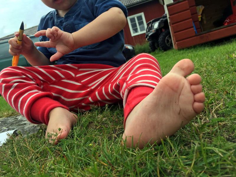
As you can see his feet are not swollen from all the bee stings they should receive according to the model. Actually, even after a week, he has not gotten a single bee sting! Which is good, I suppose, in a way, but, well, it means that my model is likely pretty crap. How can this be? Well,
- I should maybe have gotten more and better data. Perhaps the square I monitored for bumblebees didn’t yield data that was really representative of the bumblebee density in general.
- The assumption that bumblebees always sting when stepped upon might be wrong. Or maybe Torsten is so smart so that he actively avoids them…
- Maybe the model was too simplistic. I really should have made a hierarchical model incorporating data from multiple squares and several days of running around. To factor in the effect of the weather, the flower density, and the diet of Torsent also couldn’t hurt.
I guess I could spend some time improving the model. And I guess there is a lesson to be learned here about that it is hard to predict the predictive performance of a model. But all that has to wait. I am on vacation after all.
The full data and code behind this blog post can be found here.