A Bayesian Model to Calculate Whether My Wife is Pregnant or Not

On the 21st of February, 2015, my wife had not had her period for 33 days, and as we were trying to conceive, this was good news! An average period is around a month, and if you are a couple trying to go triple, then a missing period is a good sign something is going on. But at 33 days, this was not yet a missing period, just a late one, so how good news was it? Pretty good, really good, or just meh?

To get at this I developed a simple Bayesian model that, given the number of days since your last period and your history of period onsets, calculates the probability that you are going to be pregnant this period cycle. In this post I will describe what data I used, the priors I used, the model assumptions, and how to fit it in R using importance sampling. And finally I show you why the result of the model really didn’t matter in the end. Also I’ll give you a handy script if you want to calculate this for yourself. :)

The data

During the last part of 2014 my wife kept a journal of her period onsets, which was good luck for me, else I would end up with tiny data again. In total we had the dates for eight period onsets, but the data I used was not the onsets but the number of days between the onsets:

period_onset <- as.Date(c("2014-07-02", "2014-08-02", "2014-08-29", "2014-09-25", 
                          "2014-10-24", "2014-11-20", "2014-12-22", "2015-01-19"))
days_between_periods <- as.numeric(diff(period_onset))

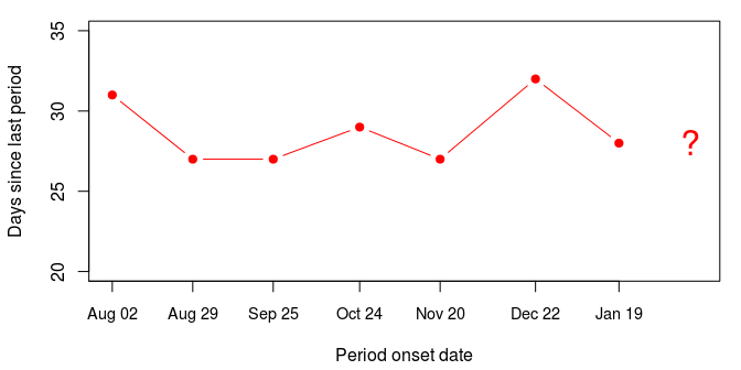
So the onsets occur pretty regularly, hovering around a cycle of 28 days. The last onset was on the 19th of January, so on the 21st of February there had been 33 days since the last onset.

Conceiving a model

I was constructing a model covering period cycles, pregnancies and infertility, and as such it was obviously going to make huge simplifications. Some general assumptions I made were:

The woman and the man have no prior reasons for being infertile as a couple.
The woman has regular periods.
The couple trying to conceive are actively trying to conceive. Say, two three times a week as recommended by Wilcox et al. (2000).
If there is pregnancy, there are no more periods.

Now to the specific assumptions I made:

The number of days between periods (days_between_periods) is assumed to be normally distributed with unknown mean (mean_period) and standard deviation (sd_period).
The probability of getting pregnant during a cycle is assumed to be 0.19 (more about where this number comes from below) if you are fertile as a couple (is_fertile). Unfortunately not all couples are fertile, and if you are not then the probability of getting pregnant is 0. If fertility is coded as 0-1 then this can be compactly written as 0.19 * is_fertile.
The probability of failing to conceive for a certain number of periods (n_non_pregnant_periods) is then (1 - 0.19 * is_fertile)^n_non_pregnant_periods
Finally, if you are not going to be pregnant this cycle, the number of days from your last to your next period (next_period) is going to be more than the current number of days since the last period (days_since_last_period). That is, the probability of next_period < days_since_last_period is zero. This sounds strange because it is so obvious, but we’re going to need it in the model.

That was basically it! But in order to fit this I was going to need a likelihood function, a function that, given fixed parameters and some data, calculates the probability of the data given those parameters or, more commonly, something proportional to a probability, that is, a likelihood. And as this likelihood can be extremely tiny I needed to calculate it on the log scale to avoid numerical problems. When crafting a log likelihood function in R, the general pattern is this:

The function will take the data and the parameters as arguments.
You initialize the likelihood to 1.0, corresponding to 0.0 on the log scale (log_like <- 0.0).
Using the probability density functions in R (such as dnorm, dbinom and dpois) you calculate the likelihoods of the different the parts of the model. You then multiply these likelihoods together. On the log scale this corresponds to adding the log likelihoods to log_like.
To make the d* functions return log likelihoods just add the argument log = TRUE. Also remember that a likelihood of 0.0 corresponds to a log likelihood of -Inf.

So, a log likelihood function corresponding to the model above would then be:

calc_log_like <- function(days_since_last_period, days_between_periods, 
                          mean_period, sd_period, next_period, 
                          is_fertile, is_pregnant) {
  n_non_pregnant_periods <- length(days_between_periods)
  log_like <- 0
  if(n_non_pregnant_periods > 0) {
    log_like <- log_like + sum( dnorm(days_between_periods, mean_period, sd_period, log = TRUE) )
  }
  log_like <- log_like + log( (1 - 0.19 * is_fertile)^n_non_pregnant_periods )
  if(!is_pregnant && next_period < days_since_last_period) {
    log_like <- -Inf
  }
  log_like
}

Here the data is the scalar days_since_last_period and the vector days_between_periods, and the rest of the arguments are the parameters to be estimated. Using this function I could now get the log likelihood for any data + parameter combination. However, I still only had half a model, I also needed priors!

Priors on periods, pregnancy and fertility

To complete this model I needed priors on all the parameters. That is, I had to specify what information the model has before seeing the data. Specifically, I needed priors on mean_period, sd_period, is_fertile, and is_pregnant (while next_period is also a parameter, I didn’t need to give it an explicit prior as its distribution is completely specified by mean_period and sd_period). I also needed to find a value for the probability of becoming pregnant in a cycle (which I set to 0.19 above). Did I use vague, “objective” priors here? No, I went looking in the fertility literature to something more informative!

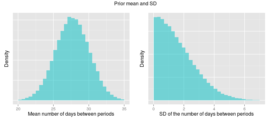
For the distribution of the days_between_periods the parameters were mean_period and sd_period. Here I used estimates from the article The normal variabilities of the menstrual cycle ( Cole et al, 2009) which measured the regularity of periods in 184 women aged 18-36 years. The grand mean number of days between periods was here 27.7 days, with the SD of the per participant mean being 2.4. The group SD of the number of days between periods was 1.6. Given these estimates I then decided to put a Normal(27.7, 2.4) distribution over mean_period and a Half-Normal distribution with mean 1.6 over sd_period, corresponding to a Half-Normal with a SD of 2.05. Here they are:

For the parameters is_fertile and is_pregnant I based the priors on frequencies. The proportion of couples that are fertile is tricky to define, as there different definitions of infertility. Van Geloven et al. (2013) made a small literature review and got that between 2% and 5% of all couples could be considered infertile. As I’ve seen numbers as high as 10%, I decided to go with the higher end of this range and put a prior probability of 100% - 5% = 95% that a couple is fertile.

is_pregnant is a binary parameter standing for whether the couple are going get (or already are) pregnant the current cycle. The prior I used here was the probability of getting pregnant in a cycle. This probability is obviously 0.0 if the couple is infertile, but how large a proportion of active, fertile couples get pregnant in a period cycle? Unfortunately I didn’t find a source that explicitly stated this, but I found something close. On page 53 in Increased Infertility With Age in Men and Women Dunson et al. (2004) give the proportion of couples trying to conceive who did not get pregnant within 12 cycles, stratified by the age of the woman:

prop_not_preg_12_cycles <- c("19-26 years" = 0.08, 
                             "27-34 years" = 0.13, 
                             "35-39 years" = 0.18)

Using some back-of-the-R-script calculations I calculated the probability to conceive in a cycle: As these proportions presumably include infertile couples I started by subtracting 0.05, the proportion of couples that I assumed are infertile. My wife was in the 27-34 years bracket so the probability of us not conceiving within 12 cycles, given that we are fertile, was then 0.13 - 0.05. If p is is the probability of not getting pregnant during one cycle, then $p^{12} = 0.13 - 0.05$ is the probability of not getting pregnant during twelve cycles and, as p is positive, we have that $p = (0.135 - 0.05)^{1/12}$. The probability of getting pregnant in one cycle is then 1 - p and the probabilities for the three age groups are:

1 - (prop_not_preg_12_cycles - 0.05)^(1/12)

## 19-26 years 27-34 years 35-39 years 
##        0.25        0.19        0.16

So that’s where the 19% percent probability of conceiving came from in the log likelihood function above, and 19% is what I used as a prior for is_pregnant. Now I had priors for all parameters and I could construct a function that returned samples from the prior:

sample_from_prior <- function(n) {
  prior <- data.frame(mean_period = rnorm(n, 27.7, 2.4),
                      sd_period   = abs(rnorm(n, 0, 2.05)),
                      is_fertile  = rbinom(n, 1, 0.95))
  prior$is_pregnant <- rbinom(n, 1, 0.19 * prior$is_fertile)
  prior$next_period <- rnorm(n, prior$mean_period, prior$sd_period)
  prior$next_period[prior$is_pregnant == 1] <- NA
  prior
}

It takes one argument (n) and returns a data.frame with n rows, each row being a sample from the prior. Let’s try it out:

sample_from_prior(n = 4)

##   mean_period sd_period is_fertile is_pregnant next_period
## 1          29      1.24          1           0          30
## 2          29      3.73          1           0          28
## 3          27      1.29          1           1          NA
## 4          27      0.57          0           0          27

Notice that is_pregnant can only be 1 if is_fertile is 1, and that there is no next_period if the couple is_pregnant.

Fitting the model using importance sampling

I had now collected the triforce of Bayesian statistics: The prior, the likelihood and the data. There are many algorithms I could have used to fit this model, but here a particularly convenient method was to use importance sampling. I’ve written about importance sampling before, but let’s recap: Importance sampling is a Monte Carlo method that is very easy to setup and that can work well if (1) the parameters space is small and (2) the priors are not too dissimilar from the posterior. As my parameter space was small and because I used pretty informative priors I though importance sampling would suffice here. The three basic steps in importance sampling are:

Generate a large sample from the prior. (This I could do using sample_from_prior.)
Assign a weight to each draw from the prior that is proportional to the likelihood of the data given those parameters. (This I could do using calc_log_like.)
Normalize the weights to sum to one so that they now form a probability distribution over the prior sample. Finally, resample the prior sample according to this probability distribution. (This I could do using the R function sample.)

(Note that there are some variations to this procedure, but when used to fit a Bayesian model this is a common version of importance sampling.)

The result of using importance sampling is a new sample which, if the importance sampling worked OK, can be treated as a sample from the posterior. That is, it represents what the model knows after having seen the data. Since I already had defined sample_from_prior and calc_log_like, defining a function in R doing importance sampling was trivial:

sample_from_posterior <- function(days_since_last_period, days_between_periods, n_samples) {
  prior <- sample_from_prior(n_samples)
  log_like <- sapply(1:n_samples, function(i) {
    calc_log_like(days_since_last_period, days_between_periods, 
                  prior$mean_period[i], prior$sd_period[i], prior$next_period[i], 
                  prior$is_fertile[i], prior$is_pregnant[i])
  })
  posterior <- prior[ sample(n_samples, replace = TRUE, prob = exp(log_like)), ]
  posterior
}

The result: probable pregnancy

So, on the 21st of February, 2015, my wife had not had her period for 33 days. Was this good news? Let’s run the model and find out!

post <- sample_from_posterior(33, days_between_periods, n_samples = 100000)

post is now a long data frame where the distribution of the parameter values represent the posterior information regarding those parameters.

head(post)

##       mean_period sd_period is_fertile is_pregnant next_period
## 33231          28       2.8          0           0          37
## 22386          27       2.4          1           1          NA
## 47489          27       2.1          1           1          NA
## 68312          28       2.3          1           1          NA
## 37341          29       2.9          1           1          NA
## 57957          30       2.6          1           0          36

Let’s start by looking at the mean and standard deviation of the number of days between each period:

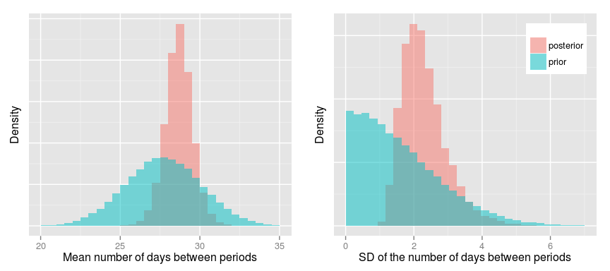
As expected the posteriors are more narrow than the priors and, looking at the posteriors, it’s probable that the mean period cycle is around 29 days with a SD of 2-3 days. Now to the important questions: What’s the probability that we are a fertile couple and what’s the probability that we were pregnant on the 21st of February? To calculate this we can just take post$is_fertile and post$is_pregnant and calculate the proportion of 1s in these vectors. A quick way of doing this is just to take the mean:

mean(post$is_fertile)

## [1] 0.97

mean(post$is_pregnant)

## [1] 0.84

So it was pretty good news: It’s very probable that we are a fertile couple and the probability that we were pregnant was 84%! Using this model I could also see how the probability of us being pregnant would change if the period onset would stay away a couple of days more:

post <- sample_from_posterior(34, days_between_periods, n_samples = 100000)
mean(post$is_pregnant)

## [1] 0.92

post <- sample_from_posterior(35, days_between_periods, n_samples = 100000)
mean(post$is_pregnant)

## [1] 0.96

Yeah, while we are at it, why not see how the probability of us being fertile and pregnant changed during the months we were trying to conceive:

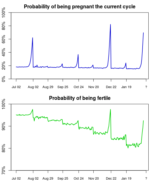
So, this make sense. As the time since the last period gets longer the probability that we are going to be pregnant the current cycle increases, but as soon as there is a period onset that probability falls down to baseline again. We see the same pattern for the probability of being fertile, but for every period cycle we didn’t get pregnant the probability of us being fertile gets slightly lower. Both these graphs are a bit jagged, but this is just due to the variability of the importance sampling algorithm. Also note that, while the graphs above are pretty, there is no real use looking at the probability over time, the only thing that’s informativ and matters is the current probability.

Some critique of the model, but which doesn’t really matter

It’s of course possible to get much better priors than my back-of-the-envelope calculation here. There are also many more predictors that one could include, like the age of the man, health factors, and so on.
The probability of getting pregnant each month could/should be made uncertain rather than giving it a fixed value, as I did. But I thought that would be one parameter to many given the little data I had.
Nothing is really normally distributed and neither is the length between periods. Here I think that assumption works well enough, but there are much more complex models of period cycle length, for example, that by Bortot et al (2010).
My model is so simple I suspect that you could almost fit it analytically. But I’m lazy and my computer is not, so importance sampling it was!

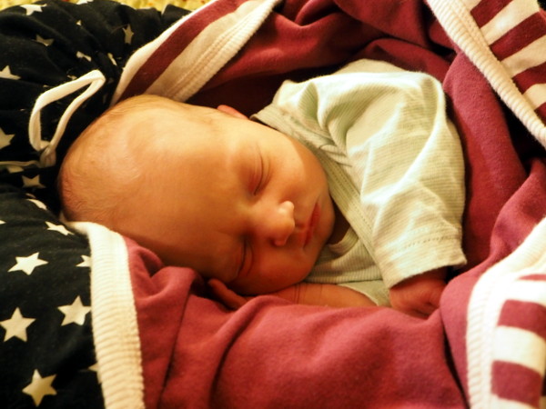
But all of this doesn’t really matter now. And the probabilities I calculated do not matter either. Before-the-fact probabilities reflect uncertainty regarding an outcome or a statement, but after-the-fact there is no uncertainty left. What uncertainty the probabilities represented is gone. I’m certain that my wife and I were pregnant on the 21st of February, and I know this because one week ago, on the 29th of October, we received this little guy:

If probabilities matter to you you can find a script implementing this model here which you can run on your own data, or a friend’s. In this post I left out the code creating the plots, but all of that can be found here. And, as this post was really just an excuse to post baby photos, here are some more of me and my son checking out the statistical literature:

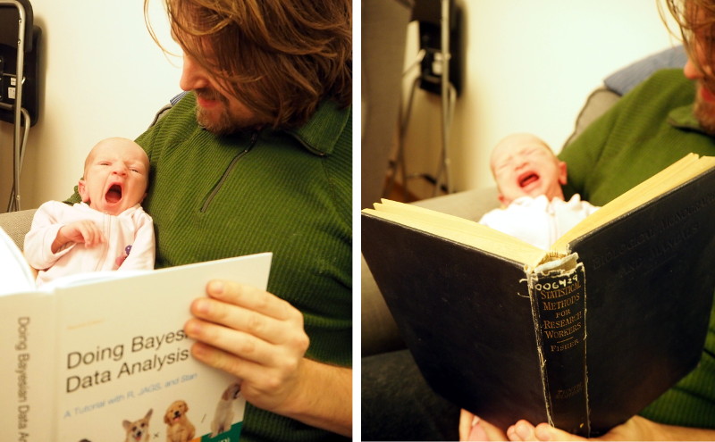
Doing Bayesian Data Analysis makes him a bit sleepy, but that’s OK, he’ll come around! Looking at Fisher’s Statistical Methods for Research Workers on the other hand makes him furious…

References

Bortot, P., Masarotto, G., & Scarpa, B. (2010). Sequential predictions of menstrual cycle lengths. Biostatistics, 11(4), 741-755. doi: 10.1093/biostatistics/kxq020

Cole, L. A., Ladner, D. G., & Byrn, F. W. (2009). The normal variabilities of the menstrual cycle. Fertility and sterility, 91(2), 522-527. doi: 10.1016/j.fertnstert.2007.11.073

Dunson, D. B., Baird, D. D., & Colombo, B. (2004). Increased infertility with age in men and women. Obstetrics & Gynecology, 103(1), 51-56. doi: 10.1097/01.AOG.0000100153.24061.45

Van Geloven, N., Van der Veen, F., Bossuyt, P. M. M., Hompes, P. G., Zwinderman, A. H., & Mol, B. W. (2013). Can we distinguish between infertility and subfertility when predicting natural conception in couples with an unfulfilled child wish?. Human Reproduction, 28(3), 658-665. doi: 10.1093/humrep/des428

Wilcox, A. J., Dunson, D., & Baird, D. D. (2000). The timing of the “fertile window” in the menstrual cycle: day specific estimates from a prospective study. Bmj, 321(7271), 1259-1262. doi: 10.1136/bmj.321.7271.1259, pdf

Posted by Rasmus Bååth | 2015-11-06 | Tags: R, Statistics, Bayesian

Publishable Stuff

Rasmus Bååth's Blog