The BASIC programming language was at one point the most widely spread programming language. Many home computers in the 80s came with BASIC (like the Commodore 64 and the Apple II), and in the 90s both DOS and Windows 95 included a copy of the QBasic IDE. QBasic was also the first programming language I encountered (I used it to write a couple of really horrible text adventures). Now I haven’t programmed in BASIC for almost 20 years and I thought I would revisit this (from my current perspective) really weird language. As I spend a lot of time doing Bayesian data analysis, I though it would be interesting to see what a Bayesian analysis would look like if I only used the tool that I had 20 years ago, that is, BASIC.
This post walks through the implementation of the Metropolis-Hastings algorithm, a standard Markov chain Monte Carlo (MCMC) method that can be used to fit Bayesian models, in BASIC. I then use that to fit a Laplace distribution to the most adorable dataset that I could find: The number of wolf pups per den from a sample of 16 wold dens. Finally I summarize and plot the result, still using BASIC. So, the target audience of this post is the intersection of people that have programmed in BASIC and are into Bayesian computation. I’m sure you are out there. Let’s go!
Getting BASIC
There are many many different version of BASIC, but I’m going for the one that I grew up with: Microsoft QBasic 1.1 . Now, QBasic is a relatively new BASIC dialect that has many advanced features such as user defined types and (gasp!) functions. But I didn’t use any fancy functions back in the 90s, and so I’m going to write old school BASIC using line numbers and GOTO, which means that the code should be relatively easy to port to, say, Commodore 64 BASIC.
Getting QBasic is easy as it seems to be freeware, and can be downloaded
here. Unless you are still using DOS, the next step would be to install
the DOSBox emulator. Once you’ve started up QBASIC.EXE you are greeted with a friendly, bright blue IDE which you can try out by entering this customary hello world script that will clear the screen and print “HELLO WORLD”.
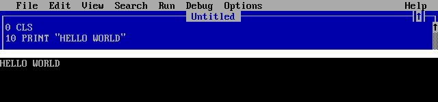
Note that in QBasic the line numbers are not strictly necessary, but in older BASICs (like the one for Commodore 64) they were necessary as the program was executed in the order given by the line numbers.
What are we going to implement?
We are going to implement the Metropolis-Hastings algorithm, a classic Markov chain Monte Carlo (MCMC) algorithm which is one of the first you’ll encounter if you study computational methods for fitting Bayesian models. This post won’t explain the actual algorithm, but the Wikipedia article is an ok introduction.
The Bayesian model we are going to implement is simple univariate Laplace distribution (just to once in awhile give the Normal distribution a day off). The Laplace is similar to the Normal distribution in that it is continuous and symmetric, but it is more peaked and has wider tails. It has two parameters: A location $\mu$, which then also defines its mean and median, and a scale $b$ which defines the width of the distribution.
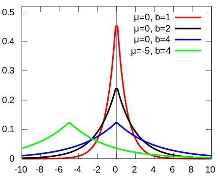
Image source, Credits:
IkamusumeFan
Like the sample mean is the maximum likelihood estimator for the mean of a Normal distribution, the sample median is the maximum likelihood estimator for the location parameter $\mu$ of a Laplace distribution. That’s why I, somewhat sloppily, think of the Normal distribution as the “mean” distribution and of the Laplace distribution as the “median” distribution. To turn this into a fully Bayesian models we need prior distributions over the two parameters. Here I’m just going to be sloppy and use a $\text{Uniform}(-\infty, \infty)$ over $\mu$ and $\log(b)$, that is, $\text{P}(\mu),\text{P}(\log(b)) \propto 1$. The full model is then
$$ x \sim \text{Laplace}(\mu, b) \\ \mu \sim \text{Uniform}(-\infty, \infty) \\ \log(b) \sim \text{Uniform}(-\infty, \infty) $$
The data we are going to use is probably the cutest dataset I’ve worked with so far. It consists of counts of the number of wolf pups in a sample of 16 wolf dens ( source):
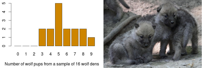
Image Source, Credits:
spacebirdy / CC-BY-SA-3.0
A reference implementation in R
Before delving into BASIC, here is a reference implementation in R of what we hope to achieve using BASIC:
# The wolf pups dataset
x <- c(5, 8, 7, 5, 3, 4, 3, 9, 5, 8, 5, 6, 5, 6, 4, 7)

# The log posterior density of the Laplace distribution model, when assuming
# uniorm/flat priors. The Laplace distribution is not part of base R but is
# available in the VGAM package.
model <- function(pars) {
  sum(VGAM::dlaplace(x, pars[1], exp(pars[2]), log = TRUE))
}

# The Metropolis-Hastings algorithm using a Uniform(-0.5, 0.5) proposal distribution
metrop <- function(n_samples, model, inits) {
  samples <- matrix(NA, nrow = n_samples, ncol = length(inits))
  samples[1,] <- inits
  for(i in 2:n_samples) {
    curr_log_dens <- model(samples[i - 1, ])
    proposal <- samples[i - 1, ] + runif(length(inits), -0.5, 0.5)
    proposal_log_dens <- model(proposal)
    if(runif(1) < exp(proposal_log_dens - curr_log_dens)) {
      samples[i, ] <- proposal
    } else {
      samples[i, ] <- samples[i - 1, ]
    }
  }
  samples
}

samples <- metrop(n_samples = 1000, model, inits = c(0,0))
# Plotting a traceplot
plot(samples[,1], type = "l", ylab = expression(Location ~ mu), col = "blue")
# Calculating median posterior and 95% CI discarding the first 250 draws as "burnin".
quantile(samples[250:1000,1], c(0.025, 0.5, 0.975))
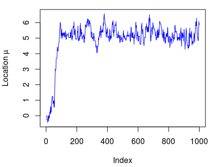
##  2.5%   50% 97.5%
## 4.489 5.184 6.144
(For the love of Markov, do not actually use this R script as a reference, it is just there to show what the BASIC code will implement. If you want to do MCMC using Metropolis-Hastings in R, check out the MCMCmetrop1R in the
MCMCpack package, or this
Metropolis-Hastings script.
R is sometimes called “a quirky language”, but the script above is a wonder of clarity and brevity compared to how the BASIC code is going to look…
Implementing the model and Metropolis-Hastings in BASIC
Let’s start by clearing the screen (CLS) and defining the variables we need. Here DIM defines arrays and matrices.
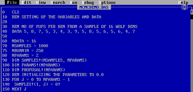
Already in this short piece of code there are a lot of fun quirkiness going on:
- As we are trying to write old school BASIC there are line numbers everywhere. This is not something that gets added automatically, they have to be written my me, and sometimes I forget a row. Hence a good strategy is to increment line numbers by 10 so that you can add missing line in between afterwards (like
75above). As there are no functions in old school BASIC the line numbers will be used to jump around in the program using statements likeGOSUBandGOTO. - ALL STATEMENTS ARE IN UPPECASE and if you write a statement in lowercase it WILL GET CORRECTED TO UPPERCASE.
- Why the exclamation mark in
SAMPLES!? In QBasic all variables are integers by default and to change the type you append a symbol to the variable name. SoTHIS$is a string whileTHAT!is a floating point number. Since our parameters are continuous most of our variables will end with a!. - The
DATAcommand is a relatively nice way to put data into the program, which can later be retrieved sequentially with theREADfunction. If you have more than one dataset? Tough luck…
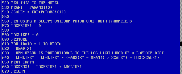
Let’s continue with defining the model. It’s going to be written as a subroutine which is an isolated piece of code that ends with a RETURN statement. It can then be called with a GOSUB <line> statement which jumps to <line>, executes the code up to the RETURN statement and then jumps back to the line after the GOSUB. It is a little bit like a poor man’s function as you can’t pass in any arguments or return any values. But that’s not a problem since all variable names are global anyway, your subroutine can still access and set any variables as long as you are careful not to use the same variable name for two different things. The subroutine below assumes that the vector PARAMS! is set and will overwrite the LOGDENS! variable. The subroutine also uses READ X! to read in a value from the DATA and RESTORE to reset the READ to the first data point.
Here is now the Metropolis-Hastings algorithm. Nothing new here, except for that we now use GOSUB 520 to jump into the model subroutine at line 520 and that we use the RND statement to generate uniformly random numbers between 0.0 and 1.0.

Summarizing it and plotting it
Now we could piece it all together by putting the following code directly after the initial declarations:

This will fill up SAMPLES! with 1000 MCMC draws from the posterior distribution of the location ($\mu$) and the log scale ($\log(b)$). But that won’t make us any happier, we still would need to summarize and plot the posterior. The code below takes the SAMPLES! matrix and calculates the mean and SD of the posterior, and a 95% credible interval (I usually prefer the median posterior and a quantile interval, but that would require much more coding, as there is no built in method for sorting arrays in BASIC.)
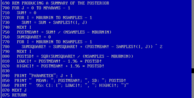
Some more BASIC strangeness here is that PRINT "HELLO", "YOU!" would produce print HELLO YOU! while PRINT "HELLO"; "YOU!" would print HELLOYOU!. That is, whether the separator is , or ; decides whether there will be a space between printed items.
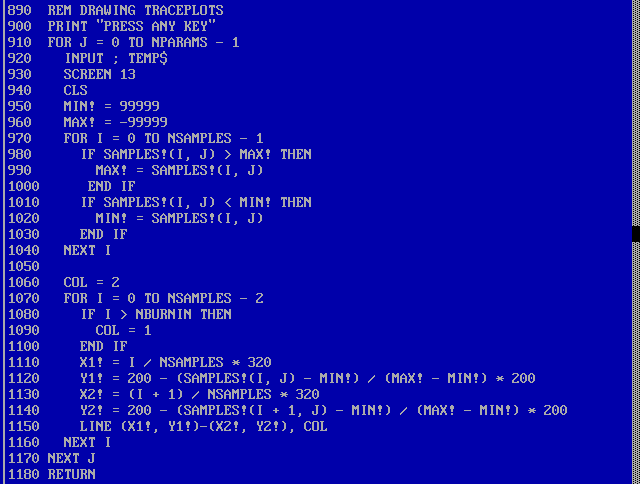
Finally we would like to draw a traceplot to make sure that the Markov chain looks ok. While there is no built in function for sorting, there is great graphics support! The bulk of the code below is mostly just rescaling the sample coordinates so that they fit the screen resolution (320 x 200). Notice also the fun syntax for drawing lines: LINE (<x1>, <y1>)-(<x2>, <y2>). That many of the BASIC statements feature “custom” syntax might be a symptom of that LINE, PRINT, IF, etc. are statements and not functions.
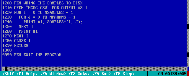
And finally we might want to write the samples to disk:
Running it
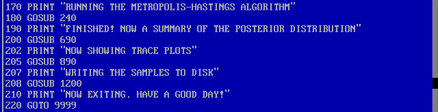
Now we are finally ready to piece everything together, sampling and plotting!
The last GOTO just jumps to the last line of the program which makes the program exit. If we set DOSBox to emulate the speed of a 33 MHz 386 PC (according to
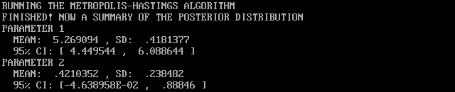
this page), it takes about a minute to generate the 1000 samples and summarize the result. Here is the output:

As drawing the lines of the traceplot is really slow we get the animation above “for free”. :)
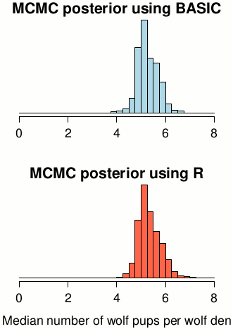
So what about the wolf pups? Well, this exercise wasn’t really about data analysis, but looking at the posterior summary above it seems like a good guess is that the median number of wolf pups in a den is around 4.5 to 6.0. I should also point out that both the BASIC code and the “reference” implementation result in similar posteriors:
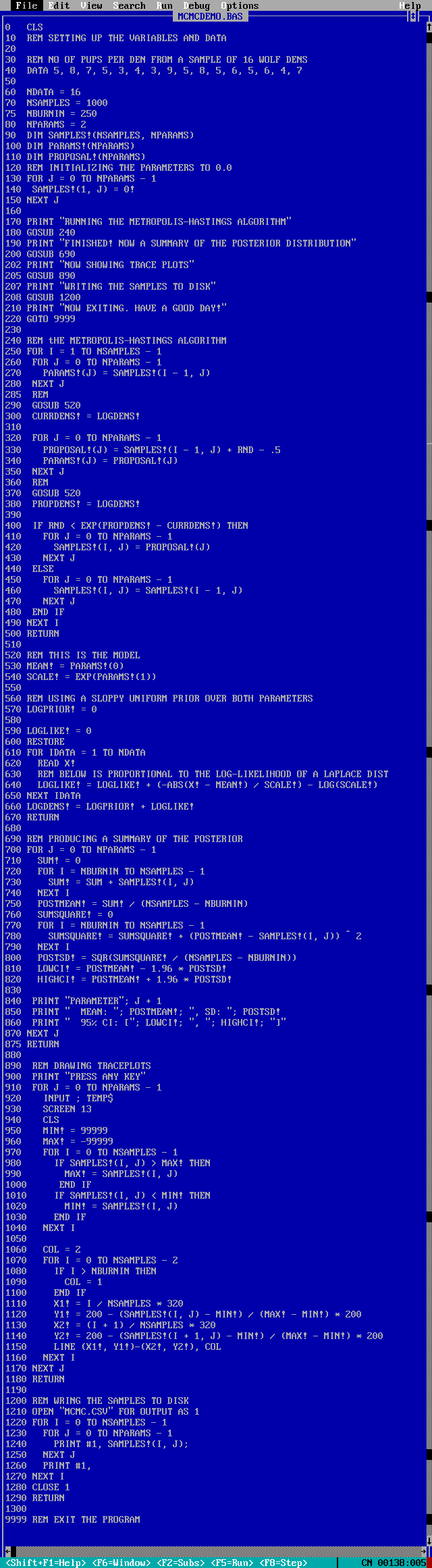
Here is the full program in text format ( MCMCDEMO.BAS), or, if you prefer, as a screenshot:
All in all, it seems like I could have done pretty advanced Bayesian statistics using the computational tools I had access to 20 years ago! (Of course, one could easily have implemented a similar program in C or FORTRAN much much earlier…) If this post has inspired you, and you wish to use BASIC as your main tool for scientific computing (please don’t!), you’ll find a host of QBasic tutorials here. You can also dive directly into the wonderful world of BASIC using this excellent javascript emulation of Apple II BASIC.
Some thoughts on BASIC
- Programming with line numbers,
GOTOandGOSUBjust feels very old school. - It is nice to not have to type a lot of brackets and parentheses all the time. (But then, on the other hand, there are a lot of verbose
END IFs andNEXT Is instead.) - Running the program above on a 386 PC was pretty quick, but it would be cool to know if it would have been possible to implement and run Metropolis-Hastings on a much slower computer, say a Commodore 64…
- It is really difficult to program when all variables live in the same global namespace! When programming this short program I still produced many bugs where I used the same variable name twice.
- BASIC isn’t one language but a set of similar languages, and while I’ve tried to write the code above using fairly old school BASIC I don’t think it would run on any other BASIC than QBasic without any modification. For example, Commodore 64 BASIC only allows you have one command following an
IF-statement, and there was noELSE! So if you wanted to execute many commands as the result of anIFstatement you would have to fake it withGOTOstatements instead. - While the QBasic language might seem a bit quirky if you are used to modern languages, the QBasic IDE is actually surprisingly friendly! Just like many modern IDEs (like, for example,
Rstudio) it has:
- Automatic syntax checking, you get direct feedback when you’ve written something wrong.
- A built in help system that works great!
- A debugger!
- An interactive prompt.
- Automatic code formatting.
print 5*5+ 7→PRINT 5 * 5 + 7