The binomial test is arguably the conceptually simplest of all statistical tests: It has only one parameter and an easy to understand distribution for the data. When introducing null hypothesis significance testing it is puzzling that the binomial test is not the first example of a test but sometimes is introduced long after the t-test and the ANOVA (as here) and sometimes is not introduced at all (as here and here). When introducing a new concept, why not start with simplest example? It is not like there is a problem with students understanding the concept of null hypothesis significance testing too well. I’m not doing the same misstake so here follows the Bayesian First Aid alternative to the binomial test!
![]()
Bayesian First Aid is an attempt at implementing reasonable Bayesian alternatives to the classical hypothesis tests in R. For the rationale behind Bayesian First Aid see the original announcement. The development of Bayesian First Aid can be followed on GitHub. Bayesian First Aid is a work in progress and I’m grateful for any suggestion on how to improve it!
The Model
Coming up with a Bayesian alternative for the binomial test is almost a no-brainer. The data is a count of the successes and failures in some task (where what is labeled success is an arbitrary choice most of the time). Given this impoverished data (no predictor variables and no dependency between trials) the distribution for the data has to be a binomial distribution with the number of Bernoulli trials ($n$) fixed and the relative frequency of success ($\theta$) as the only free parameter. Notice that $\theta$ is often called the probability of success but from a Bayesian perspective I believe this is almost a misnomer and, at the very least, a very confusing name. The result of a Bayesian analysis is a probability distribution over the parameters and calling $\theta$ a probability can result in hard-to-decipher statements like: “The probability that the probability is larger than 50% is more than 50%”. Calling $\theta$ the relative frequency of success also puts emphasis on that $\theta$ is a property of a process and reserves “probability” for statements about knowledge (keeping probabilities nicely “inside the agent”).
The only part of the model that requires some thought is the prior distribution for $\theta$. There seems to mainly be three priors that are proposed as non-informative distributions for $\theta$: The flat prior, Jeffrey’s’ prior and Haldanes prior. These priors are beautifully described by Zhu and Lu (2004) and the flat and Jeffrey’s are pictured below.

The Haldane prior is trickier to visualize as it puts an infinite amount of mass at $\theta=0$ and $\theta=1$.
As explained by Zhu and Lu, the Haldane prior could be considered the least informative prior, so isn’t that what we want? Nope, I’ll go with the flat distribution which can also be considered as “lest informative” when we know that both successes and failures are possible (Lee, 2004). I believe that in most cases when binomial data is analyzed it is known (or at least suspected) a priori that both successes and failures are possible thus it makes sense to use the flat prior as the default prior.
The flat prior is conveniently constructed as a $\mathrm{Beta}(1,1)$ distribution. A $\mathrm{Uniform}(0,1)$ could equally well be used but the $\mathrm{Beta}$ has the advantage that it is easy to make it more or less informative by changing the two parameters. For example, if you want to use Jeffrey’s prior instead of the flat you would use a $\mathrm{Beta}(0.5,0.5)$ and a Haldane prior can be approximated by $\mathrm{Beta}(\epsilon,\epsilon)$ where $\epsilon$ is close to zero, say 0.0001.
The final Bayesian First Aid alternative to the binomial test is then:
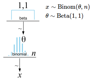
The diagram to the left is a Kruschke style diagram. For an easy way of making such a diagram check out this post.
The bayes.binom.test function
Having a model is fine but Bayesian First Aid is also about being able to run the model in a nice way and getting useful output. First let’s find some binomial data and use it to run a standard binomial test in R. The highly cited Nature paper Poleward shifts in geographical ranges of butterfly species associated with regional warming describes how the geographical areas of a sample of butterfly species have moved northwards, possibly as an effect of the rising global temperature. In that paper we find the following binomial data:

Here is the corresponding binomial test in R with “retracting northwards” as success and “extending southwards” as failure:
binom.test(c(9, 2))
##
## 	Exact binomial test
##
## data:  c(9, 2)
## number of successes = 9, number of trials = 11, p-value = 0.06543
## alternative hypothesis: true probability of success is not equal to 0.5
## 95 percent confidence interval:
##  0.4822 0.9772
## sample estimates:
## probability of success
##                 0.8182
Not a significant result at the 5% $\alpha$ level. C’est la vie.
Fun fact: The resulting p-value is not the same as that reported in the Nature paper. By closer inspection it seems like the reported p-value is correct as Table 2 shows that there actually were ten species retracting northwards and not nine, “9 retracting north” was a typo and should have read “10 retracting north”. I leave it as an excecise for the interested reader to find the other wrongly reported binomial test p-value in the paper. Despite being a typo, here I’ll continue with nine successes and two failures.
Now to run the Bayesian First Aid alternative you simply prepend bayes. to the function call.
library(BayesianFirstAid)
bayes.binom.test(c(9, 2))
##
## 	Bayesian first aid binomial test
##
## data: c(9, 2)
## number of successes = 9, number of trials = 11
## Estimated relative frequency of success:
##   0.769
## 95% credible interval:
##   0.554 0.964
## The relative frequency of success is more than 0.5 by a probability of 0.981
## and less than 0.5 by a probability of 0.019
I’ve chosen to make the output similar to binom.test. You get to know what data you put in, you get a point estimate (here the mean of the posterior of $\theta$) and you get a credible interval. You don’t get a p-value, you do get the probability that $\theta$ is lower or higher that a comparison value which defaults to 0.5. Looking at these probabilities and the credible interval it seems like there is pretty good evidence that butterflies are generally moving northwards.
A goal with Bayesian First Aid is complete compliance with the calling structure of the original test functions. You should be able to use the same arguments in the same way as you are used to with binom.test. For example, the call
binom.test(9, 11, conf.level = 0.8, p = 0.75, alternative = "greater")
is handled by bayes.binom.test by using an 80% credible interval and using 0.75 as the comparison value. I haven’t figured out anything useful to do with alternative="greater" so that simply issues a warning:
bayes.binom.test(9, 11, conf.level = 0.8, p = 0.75, alternative = "greater")
## Warning: The argument 'alternative' is ignored by bayes.binom.test
##
## 	Bayesian first aid binomial test
##
## data: 9 and 11
## number of successes = 9, number of trials = 11
## Estimated relative frequency of success:
##   0.769
## 80% credible interval:
##   0.647 0.925
## The relative frequency of success is more than 0.75 by a probability of 0.609
## and less than 0.75 by a probability of 0.391
If you run the same call to bayes.binom.test repeatedly you’ll notice that you get slightly different values every time. This is because Markov chain Monte Carlo (MCMC) approximation is used to approximate the posterior distribution of $\theta$. The accuracy of the MCMC approximation is governed by the n.iter parameter which defaults to 15000. This should be enough for most purposes but if you feel it is not enough, just max it up!
bayes.binom.test(c(9, 2), n.iter = 999999)
Generic Functions
Every Bayesian First Aid test have corresponding plot, summary, diagnostics and model.code functions.
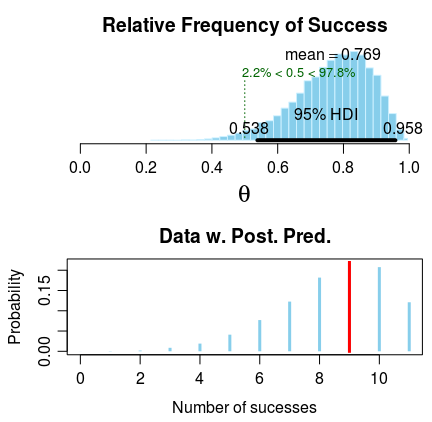
plot plots the parameters of interest and, if appropriate, a
posterior predictive distribution. In the case of bayes.binom.test there is just one parameter $\theta$. The plot of the posterior is a design by John D. Kruschke copied from his
Bayesian estimation supersedes the t test program. To get the plot, first save the output of bayes.binom.test to a variable and then plot it!
fit <- bayes.binom.test(c(9, 2))
plot(fit)
summary prints out a comprehensive summary of all the parameters in the model:
summary(fit)
##   Data
## number of successes = 9, number of trials = 11
##
##   Model parameters and generated quantities
## theta: The relative frequency of success
## x_pred: Predicted number of successes in a replication
##
##   Measures
##         mean    sd HDIlo  HDIup %<comp %>comp
## theta  0.769 0.114 0.538  0.958  0.022  0.978
## x_pred 8.462 1.830 5.000 11.000  0.000  1.000
##
## 'HDIlo' and 'HDIup' are the limits of a 95% HDI credible interval.
## '%<comp' and '%>comp' are the probabilities of the respective parameter being
## smaller or larger than 0.5.
##
##   Quantiles
##        q2.5%  q25% median   q75% q97.5%
## theta  0.508 0.698  0.783  0.855  0.945
## x_pred 4.000 7.000  9.000 10.000 11.000
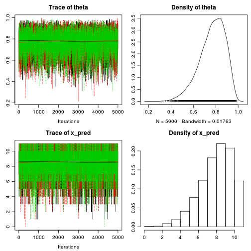
diagnostics prints and plots MCMC diagnostics calculated using the
coda package. In the case of bayes.binom.test MCMC diagnostics is overkill, still it is nice to get that warm fuzzy feeling you get when looking at converging MCMC chains:
diagnostics(fit)
##
## Iterations = 1:5000
## Thinning interval = 1
## Number of chains = 3
## Sample size per chain = 5000
##
##   Diagnostic measures
##         mean    sd mcmc_se n_eff  Rhat
## theta  0.769 0.114   0.001 14795 1.000
## x_pred 8.462 1.830   0.015 14787 1.001
##
## mcmc_se: the estimated standard error of the MCMC approximation of the mean.
## n_eff: a crude measure of effective MCMC sample size.
## Rhat: the potential scale reduction factor (at convergence, Rhat=1).
##
##   Model parameters and generated quantities
## theta: The relative frequency of success
## x_pred: Predicted number of successes in a replication
Last but not least model.code prints out R and JAGS code that runs the model and that you can copy-n-paste directly into an R script:
model.code(fit)
## ### Model code for the Bayesian First Aid alternative to the binomial test ###
## require(rjags)
##
## # Setting up the data
## x <- 9
## n <- 11
##
## # The model string written in the JAGS language
## model_string <-"model {
##   x ~ dbinom(theta, n)
##   theta ~ dbeta(1, 1)
##   x_pred ~ dbinom(theta, n)
## }"
##
## # Running the model
## model <- jags.model(textConnection(model_string), data = list(x = x, n = n),
##                     n.chains = 3, n.adapt=1000)
## samples <- coda.samples(model, c("theta", "x_pred"), n.iter=5000)
##
## # Inspecting the posterior
## plot(samples)
## summary(samples)
For example, in order to change the flat prior on $\theta$ into Jeffrey’s prior we simply change dbeta(1, 1) into dbeta(0.5, 0.5) and rerun the code:
x <- 9
n <- 11

model_string <-"model {
  x ~ dbinom(theta, n)
  theta ~ dbeta(0.5, 0.5)
  x_pred ~ dbinom(theta, n)
}"

model <- jags.model(textConnection(model_string), data = list(x = x, n = n),
                    n.chains = 3, n.adapt=1000)
## Compiling model graph
##    Resolving undeclared variables
##    Allocating nodes
##    Graph Size: 5
##
## Initializing model
samples <- coda.samples(model, c("theta", "x_pred"), n.iter=5000)

summary(samples)
##
## Iterations = 1:5000
## Thinning interval = 1
## Number of chains = 3
## Sample size per chain = 5000
##
## 1. Empirical mean and standard deviation for each variable,
##    plus standard error of the mean:
##
##         Mean    SD Naive SE Time-series SE
## theta  0.792 0.113 0.000919       0.000926
## x_pred 8.717 1.791 0.014626       0.014594
##
## 2. Quantiles for each variable:
##
##         2.5%   25%   50%    75%  97.5%
## theta  0.536 0.723 0.809  0.877  0.961
## x_pred 5.000 8.000 9.000 10.000 11.000