Anscombe’s quartet is a collection of four datasets that look radically different yet result in the same regression line when using ordinary least square regression. The graph below shows Anscombe’s quartet with imposed regression lines (taken from the Wikipedia article).

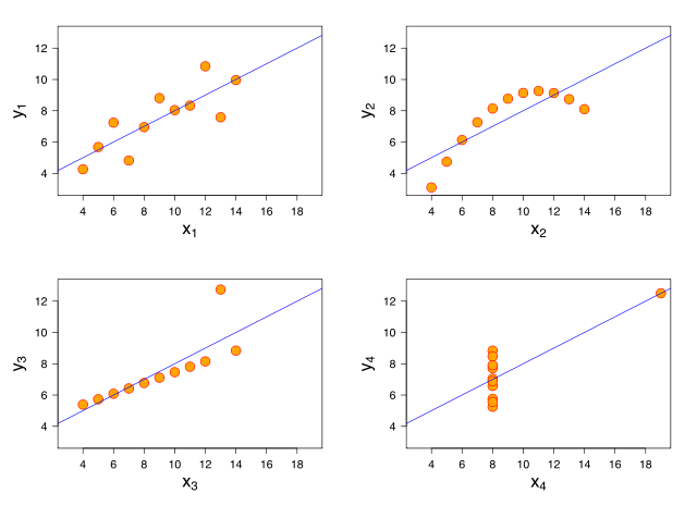
While least square regression is a good choice for dataset 1 (upper left plot) it fails to capture the shape of the other three datasets. In a recent post John Kruschke shows how to implement a Bayesian model in JAGS that captures the shape of both data set 1 and 3 (lower left plot). Here I will expand that model to capture the shape of all four data sets. If that sounds interesting start out by reading Kruschke’s post and I will continue where that post ended…

Ok, using a wide tailed t distribution it was possible to down weight the influence of the outlier in dataset 3 while still capturing the shape of dataset 1. It still fails to capture datasets 2 and 4 however. Looking at dataset 2 (upper right plot) it is clear that we would like to model this as a quadratic curve and what we would like to do is to allow the model to include a quadratic term when the data supports it (as dataset 2 does) and refrain from including a quadratic term when the data supports a linear trend (as in datasets 1 and 3). A solution is to include a quadratic term (b2) with a spike and slab prior distribution which is a mixture between two distributions one thin (spiky) distribution and one wide (slab) distribution. By centering the spike over zero we introduce a bit of automatic model selection into our model, that is, if there is evidence for a quadratic trend in the data then the slab will allow this trend to be included in the model, however, if there is little evidence for a quadratic trend then the spike will make the estimate of b2 practically equivalent to zero. In JAGS such a prior can be implemented as follows:

b2 <- b2_prior[b2_pick + 1]
b2_prior[1] ~ dnorm(0, 99999999999999) # spike
b2_prior[2] ~ dnorm(0, 0.1) # slab
b2_pick ~ dbern(0.5)

The argument to the dbern function indicates our prior belief that the data includes a quadratic term, in this case we think the odds are 50/50. The resulting prior looks like this:

How to model dataset 4? Well, I don’t think it is clear what dataset 4 actually shows. Since there are many datapoints at x = 8 we should be pretty sure about the mean and SD at that point. Otherwise the only datapoint is that at x = 19 and this really doesn’t tell much. For me, a good description of dataset 4 would be lots of certainty at x = 8 and lots of uncertainty for any other value of x. One reason why ordinary least squares regression doesn’t work here is because of the assumption that the variance of the data (y) is the same at any x. The many datapoints at x = 8 also make an ordinary least squares regression very certain about the variance at x = 19. By allowing the variance to vary at different x we can implement a model that isn’t overconfident regarding the variance at x = 19. The following JAGS code implements a variance (here reparameterized as precision) that can differ at different x:

tau[i] <- exp( t0_log + t1_log * x[i] )
t0_log ~ dunif(-10, 10)
t1_log ~ dunif(-10, 10)

Putting everything together in one JAGS model and using R and rjags to run it:

library(datasets)
library(rjags)

model_string <- "
model{
for(i in 1:length(x)) {
  y[i] ~ dt( b0 + b1 * x[i] + b2 * pow(x[i], 2), tau[i], nu )
  tau[i] <- exp( t0_log + t1_log * x[i] )
}
nu <- nuMinusOne + 1
nuMinusOne ~ dexp( 1/29 )
b0 ~ dnorm(0, 0.0001)
b1 ~ dnorm(0, 0.0001)
b2 <- b2_prior[b2_pick + 1]
b2_prior[1] ~ dnorm(0, 99999999999999)
b2_prior[2] ~ dnorm(0, 0.1)
b2_pick ~ dbern(0.5)
t0_log ~ dunif(-10, 10)
t1_log ~ dunif(-10, 10)
}
"

Now lets see how this model performs on the Anscombe’s quartet. The following runs the model for dataset 1:

m <- jags.model(textConnection(model_string),
  list(x = anscombe$x1, y = anscombe$y1), n.adapt=10000)
update(m, 10000)
s <- coda.samples(m,
  c("b0", "b1", "b2", "t0_log", "t1_log","b2_pick"), n.iter=20000)
plot(s)

Resulting in the following traceplots and parameter estimates:

Looks reasonable enough, there seems to be little evidence for a quadratic trend in the data. Now lets plot the data with 40 randomly chosen regression lines from the MCMC samples superimposed:

samples_mat <- as.matrix(samples)
plot(anscombe$x1, anscombe$y1, xlim=c(0, 20),
  ylim=c(0, 20), pch=16, xlab="X", ylab="Y")
for(row_i in sample(nrow(samples_mat), size=40)) {
  curve(samples_mat[row_i,"b0"] + samples_mat[row_i,"b1"] * x +
    samples_mat[row_i,"b2"] * x^2, 0, 20, add=T, col=rgb(0.3, 0.3, 1, 0.5))
}

Also looks reasonable. Now lets do the same for the three other datasets. Dataset 2:

Well, the trace plots looks a bit strange but this is because the data is a perfect quadratic function with no noise which the model is able to capture as the superimposed regression lines look the same.

Now for dataset 3:

This works well too! The superimposed regression lines are not influenced by the outlier just as in Kruschke’s model.

At last, dataset 4:

Well, the trace plots look a bit strange even if I run the model for a large amount of samples (the plots above show 1 000 000 samples). The resulting regression lines are also difficult to interpret, a lot of them go through the point at x = 19 but there are also many lines that are far off. Still I believe it better captures how I view dataset 4, that is, it might be that there is a strong increasing trend as shown by the datapoint at x = 19 but any other trend is actually also possible.

To conclude. I think it is really cool how crazy models it is possible to build using Bayesian modeling and JAGS. I mean, the model I’ve presented here is not really sane and I would not use it for anything serious. For one thing, it seems to be quite sensitive to the priors (yes, guilty guilty, I had to tamper with the priors a little bit to get it to work…).

From my perspective, the above exercise shows a difference between classical statistics and Bayesian statistics. Using classical statistics it would be quite difficult to implement the model above. “Please use a normal distribution and maybe transform the data, if you must.” – Classical statistics. Bayesian statistics is more easy going, I can use whatever distribution I want and building a model is like building a LEGO castle. “Hey, why don’t you try using a t brick for the towers? And while you’re at it, put a spiky slab brick on top, it will look like a flagpole!” – Bayesian statistics.