In the last blog post I showed my initial attempt at modeling football results in La Liga using a Bayesian Poission model, but there was one glaring problem with the model; it did not consider the advantage of being the home team. In this post I will show how to fix this! I will also show a way to deal with the fact that the dataset covers many La Liga seasons and that teams might differ in skill between seasons.
Modeling Match Results: Iteration 2
The only change to the model needed to account for the home advantage is to split the baseline into two components, a home baseline and an away baseline. The following JAGS model implements this change by splitting baseline into home_baseline and away_baseline.
# model 2
m2_string <- "model {
for(i in 1:n_games) {
  HomeGoals[i] ~ dpois(lambda_home[HomeTeam[i],AwayTeam[i]])
  AwayGoals[i] ~ dpois(lambda_away[HomeTeam[i],AwayTeam[i]])
}

for(home_i in 1:n_teams) {
  for(away_i in 1:n_teams) {
    lambda_home[home_i, away_i] <- exp( home_baseline + skill[home_i] - skill[away_i])
    lambda_away[home_i, away_i] <- exp( away_baseline + skill[away_i] - skill[home_i])
  }
}

skill[1] <- 0
for(j in 2:n_teams) {
  skill[j] ~ dnorm(group_skill, group_tau)
}

group_skill ~ dnorm(0, 0.0625)
group_tau <- 1/pow(group_sigma, 2)
group_sigma ~ dunif(0, 3)

home_baseline ~ dnorm(0, 0.0625)
away_baseline ~ dnorm(0, 0.0625)
}"
Another cup of coffee while we run the MCMC simulation…
m2 <- jags.model(textConnection(m2_string), data = data_list, n.chains = 3,
    n.adapt = 5000)
update(m2, 5000)
s2 <- coda.samples(m2, variable.names = c("home_baseline", "away_baseline",
    "skill", "group_sigma", "group_skill"), n.iter = 10000, thin = 2)
ms2 <- as.matrix(s2)
Looking at the trace plots and distributions of home_baseline and away_baseline shows that there is a considerable home advantage.
plot(s2[, "home_baseline"])

plot(s2[, "away_baseline"])

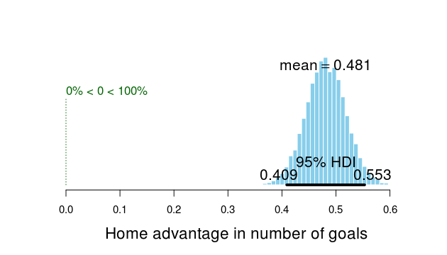
Looking at the difference between exp(home_baseline) and exp(away_baseline) shows that the home advantage is realized as roughly 0.5 more goals for the home team.
plotPost(exp(ms2[, "home_baseline"]) - exp(ms2[, "away_baseline"]), compVal = 0,
    xlab = "Home advantage in number of goals")
Comparing the DIC of the of the two models also indicates that the new model is better.
dic_m1 <- dic.samples(m1, 10000, "pD")
dic_m2 <- dic.samples(m2, 10000, "pD")
diffdic(dic_m1, dic_m2)
## Difference: 167
## Sample standard error: 26.02
Finally we’ll look at the simulated results for Valencia (home team) vs Sevilla (away team) using the estimates from the new model with the first row of the graph showing the predicted outcome and the second row showing the actual data.
plot_pred_comp2 <- function(home_team, away_team, ms) {
    par(mfrow = c(2, 4))
    home_baseline <- ms[, "home_baseline"]
    away_baseline <- ms[, "away_baseline"]
    home_skill <- ms[, col_name("skill", which(teams == home_team))]
    away_skill <- ms[, col_name("skill", which(teams == away_team))]
    home_goals <- rpois(nrow(ms), exp(home_baseline + home_skill - away_skill))
    away_goals <- rpois(nrow(ms), exp(away_baseline + away_skill - home_skill))
    plot_goals(home_goals, away_goals)
    home_goals <- d$HomeGoals[d$HomeTeam == home_team & d$AwayTeam == away_team]
    away_goals <- d$AwayGoals[d$HomeTeam == home_team & d$AwayTeam == away_team]
    plot_goals(home_goals, away_goals)
}

plot_pred_comp2("FC Valencia", "FC Sevilla", ms2)

And similarly Sevilla (home team) vs Valencia (away team).
plot_pred_comp2("FC Sevilla", "FC Valencia", ms2)

Now the results are closer to the historical data as both Sevilla and Valencia are more likely to win when playing as the home team.
At this point in the modeling process I decided to try to split the skill parameter into two components, offence skill and defense skill, thinking that some teams might be good at scoring goals but at the same time be bad at keeping the opponent from scoring. This didn’t seem to result in any better fit however, perhaps because the offensive and defensive skill of a team tend to be highly related. There is however one more thing I would like to change with the model…
Modeling Match Results: Iteration 3
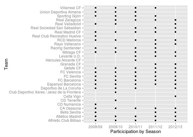
The data set laliga contains data from five different seasons and an assumption of the current model is that a team has the same skill during all seasons. This is probably not a realistic assumption, teams probably differ in their year-to-year performance. And what more, some teams do not even participate in all seasons in the laliga data set, as a result of dropping out of the first division, as the following diagram shows:
qplot(Season, HomeTeam, data = d, ylab = "Team", xlab = "Particicipation by Season")
The second iteration of the model was therefore modified to include the year-to-year variability in team skill. This was done by allowing each team to have one skill parameter per season but to connect the skill parameters by using a team’s skill parameter for season $t$ in the prior distribution for that team’s skill parameter for season $t+1$ so that
$$\text{skill}{t+1} \sim \text{Normal}(\text{skill}{t}, \sigma_{\text{season}}^2)$$
for all different $t$, except the first season which is given an vague prior. Here $\sigma_{\text{season}}^2$ is a parameter estimated using the whole data set. The home and away baselines are given the same kind of priors and below is the resulting JAGS model.
m3_string <- "model {
for(i in 1:n_games) {
  HomeGoals[i] ~ dpois(lambda_home[Season[i], HomeTeam[i],AwayTeam[i]])
  AwayGoals[i] ~ dpois(lambda_away[Season[i], HomeTeam[i],AwayTeam[i]])
}

for(season_i in 1:n_seasons) {
  for(home_i in 1:n_teams) {
    for(away_i in 1:n_teams) {
      lambda_home[season_i, home_i, away_i] <- exp( home_baseline[season_i] + skill[season_i, home_i] - skill[season_i, away_i])
      lambda_away[season_i, home_i, away_i] <- exp( away_baseline[season_i] + skill[season_i, away_i] - skill[season_i, home_i])
    }
  }
}

skill[1, 1] <- 0
for(j in 2:n_teams) {
  skill[1, j] ~ dnorm(group_skill, group_tau)
}

group_skill ~ dnorm(0, 0.0625)
group_tau <- 1/pow(group_sigma, 2)
group_sigma ~ dunif(0, 3)

home_baseline[1] ~ dnorm(0, 0.0625)
away_baseline[1] ~ dnorm(0, 0.0625)

for(season_i in 2:n_seasons) {
  skill[season_i, 1] <- 0
  for(j in 2:n_teams) {
    skill[season_i, j] ~ dnorm(skill[season_i - 1, j], season_tau)
  }
  home_baseline[season_i] ~ dnorm(home_baseline[season_i - 1], season_tau)
  away_baseline[season_i] ~ dnorm(away_baseline[season_i - 1], season_tau)
}

season_tau <- 1/pow(season_sigma, 2)
season_sigma ~ dunif(0, 3)
}"
These changes to the model unfortunately introduces quit a lot of autocorrelation when running the MCMC sampler and thus I increase the number of samples and the amount of thinning. On my setup the following run takes the better half of a lunch break (and it wouldn’t hurt to run it even a bit longer).
m3 <- jags.model(textConnection(m3_string), data = data_list, n.chains = 3,
    n.adapt = 10000)
update(m3, 10000)
s3 <- coda.samples(m3, variable.names = c("home_baseline", "away_baseline",
    "skill", "season_sigma", "group_sigma", "group_skill"), n.iter = 40000,
    thin = 8)
ms3 <- as.matrix(s3)
The following graph shows the trace plot and distribution of the season_sigma parameter.
plot(s3[, "season_sigma"])

Calculating and comparing the DIC of this model with the former model show no substantial difference.
dic_m3 <- dic.samples(m3, 40000, "pD")
diffdic(dic_m2, dic_m3)
## Difference: 13.73
## Sample standard error: 9.575
However, I believe the assumptions of the current model (m3) are more reasonable so I’ll stick with this model. In part three of Modeling Match Results in La Liga Using a Hierarchical Bayesian Poisson Model I will use my model to complete the goals set out in the introduction. That is, ranking the teams in La Liga and predicting the outcome of future matches.